TBA 4125 - Prosjektering - Konstruksjon
Spring 2023
Lecture 0 - Course Introduction
The learning goal of today is:
- getting started
- become aware about the practicalities of the course
- become aware about the priciple content of the course
Reading / Homework:
- Reading the lecture notes distributed on BlackBoard (Lecture 0 and 1)
- Per Kr. Larsen - Konstruksjonsteknikk: Chapters 1 + 2 (optional)
Some general practicalities
Lectures and exercises will take place Wednesdays 08-10 *online* and Thursdays 08-10 *VE1*.
Lectures and exercises will be held by:
- Jochen Köhler:
- Materialteknisk 3-209/ jochen.kohler@ntnu.no
The following course related material can be found on Blackboard:
- Lecture Notes
- Lecture Slides
- Exercises
- Exercise Solutions
- Supplemental Material
- Announcements
Learning Strategy:
- Students are entitled to read the announced homeworkmaterial before the lecture.
- The lecture is used to briefly summarize the reading material, answer questions and demonstrate examples.
Students have to engage in 3 compulsory exercises and 1 project work. The project work is intended to be a group work.
Preliminary lecture plan 2023:
| Date | Topic |
| Wed 11.1. | K-00: Introduction to the course, practicalities |
| Thu 12.1. | K-01: Introduction to structural design |
| Wed 18.1. | K-02: Understanding Structures |
| Thu 19.1. | K-03: Principle load effects on structures (Part 1) |
| Wed 25.1. | K-04: Principle load effects on structures (Part 2) |
| Thu 26.1. | K-05: Loads on structures, snow loads |
| Wed 01.2. | K-06: Wind loads |
| Thu 02.2. | K-07: Safety and Structural Reliability |
| Wed 08.2. | K-08: Exercises |
| Thu 09.2. | K-09: Semi-Probabilistic Design concept |
| Wed 15.2. | K-10: Semi-Probabilistic Design according to the EUROCODES |
Preliminary plan of assignments 2023:
| Assignments | Start | Due (Frist) |
| 1. Load bearing systems | 19.1 | 28.1. |
| 2. Loads on structures | 29.1. | 08.2. |
| 3. Reliability | 09.2. | 18.2. |
| Project work | 09.2. | 11.3.(1500h) |
Additional reading resources:
- Per Kristian Larsen— Konstruksjonsteknikk, Laster og bæresystemer
- We will have special emphasis to chapters 1 -5
- Can be ordered via Fagbokforlaget
Figure 1

- Jörg Schneider— Introduction to Safety and Reliability of Structures
- We have special emphasis to chapter 4.3
- Is available online via NTNU Library
Figure 2
- The EUROCODES, in particular:
- NS EN1990 (Basis of Design)
- NS EN1991 (Loads)
- Available online via NTNU Library
Figure 3

- EUROCODE— background document
- Interesting background information and examples
- Available online via NTNU Library
Figure 4
Introduction to Structural Engineering
Civil Engineers play an important role in our society. Many current and future challenges, as related to the efficient management of (limited) financial and natural resources or the appropriate mitigation to the possible effects of climate change, are closely related to the built environment and require good civil engineering. As the challenges will increase, the demand for new and innovative solutions, i.e. well beyond traditional engineering practice, will increase. The role of future civil engineers is very nicely defined by the American Society of Civil Engineers (ASCE) as a professional who is:
Entrusted by society to create a sustainable world and enhance the global quality of life. Civil engineers serve competently, collaboratively, and ethically as master:
- planners, designers, constructors, and operators of society’s economic and social engine, the built environment;
- stewards of the natural environment and its resources;
- innovators and integrators of ideas and technology across the public, private, and academic sectors;
- managers of risk and uncertainty caused by natural events, accidents, and other threats; and
- leaders in discussions and decisions shaping public environmental and infrastructure policy.
1: ASCE is the permanent organisation representing the civil engineering profession in the United States.
The planning, design, maintenance and construction of structures plays a key role in the general civil engineering area and the engineering discipline dedicated to structures is called Structural Engineering.
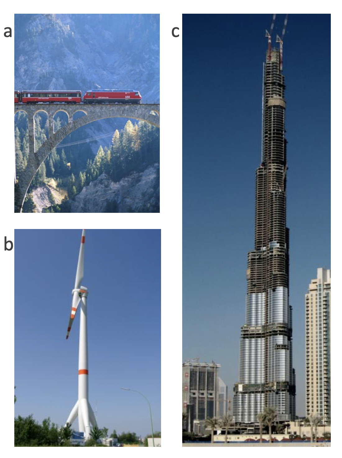
Structures are the "bones and muscles" of the built environment. They are intended to bear loads and enable all kinds of societal utility by creating sheltered space (e.g. buildings), supporting infrastructure (e.g. bridges) or facilitate industrial or energy production (e.g. wind turbines), see figure 1. Thereby, structures have played and will play a key role for successful societal development.
At the same time structures are responsible for the consumption of large amounts of natural and economic resources. The construction industry is responsible for an overall share of around 40% of total energy consumption, 90% of global raw materials usage (in tons). Moreover, in most developed countries the construction industry contributes with 10% or more to the GDP and constitutes a key prerequisite for all critical infrastructures, including transport, communication, energy, production, food and housing.
A solid basic understanding of structural engineering principles is paramount for all cilvil engineers that work in connection to the built environment. The transfer of the most basic principles is the objective of this part of the course. The topics adressed in the course therefore are:
- Principle load bearing systems
- Attaining structural requirements, structural safety
- Representation of loads on structures
Figure 5: Structures can look very different but they all support important societal activities - and they transfer loads into the ground. a. Railwaybridge, Switzerland; b. Windenergyconverter; c. Burj Khalifa (828m), Dubai. --------------
Lecture 1 - The structural engineering design process
The learning goal of today is:
- gaining principle understanding of the structural design process
- get an understanding of the principle steps and corresponding challenges
Reading / Homework:
- Reading the lecture notes distributed on BlackBoard (Lecture 2)
- Per Kr. Larsen - Konstruksjonsteknikk: Chapters 1 + 2
Design of a roof - a motivating example
Figure 6: A flat roof is often exposed to considerable snow loads.
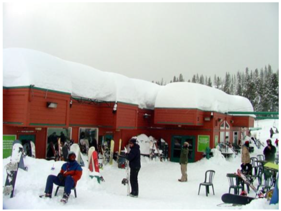
In order to demonstrate the principle challenges of a structural design process let's consider a typical structural design situation as an example:
A flat roof exposed to snow load has to be designed.
Any experienced structural engineer would follow a rather standardised procedure to do the job. However, let's assume we do this the first time and just use our already developed engineering understanding to identify a systematic approach for solving this problem.
So, how could we start, what would be the first step?
1. Context and requirements: Prior to any analysis we have to clarify some principle questions with regard to the requirements to the structure. The dimensions of the space that has to be sheltered is generally specified / required by the client. E.g. the client might specify that the required roof area is 20x8 square-meters. Furthermore the client has to specify what he expects from the roof in regard to its load bearing behaviour. Generally a client expects a (roof-) structure to be:
- safe - it should carry the load and not fail,
- sufficiently stiff - i.e. it should not deform extensively (as this would jeopardise the functionality of the roof).
- cost efficient .
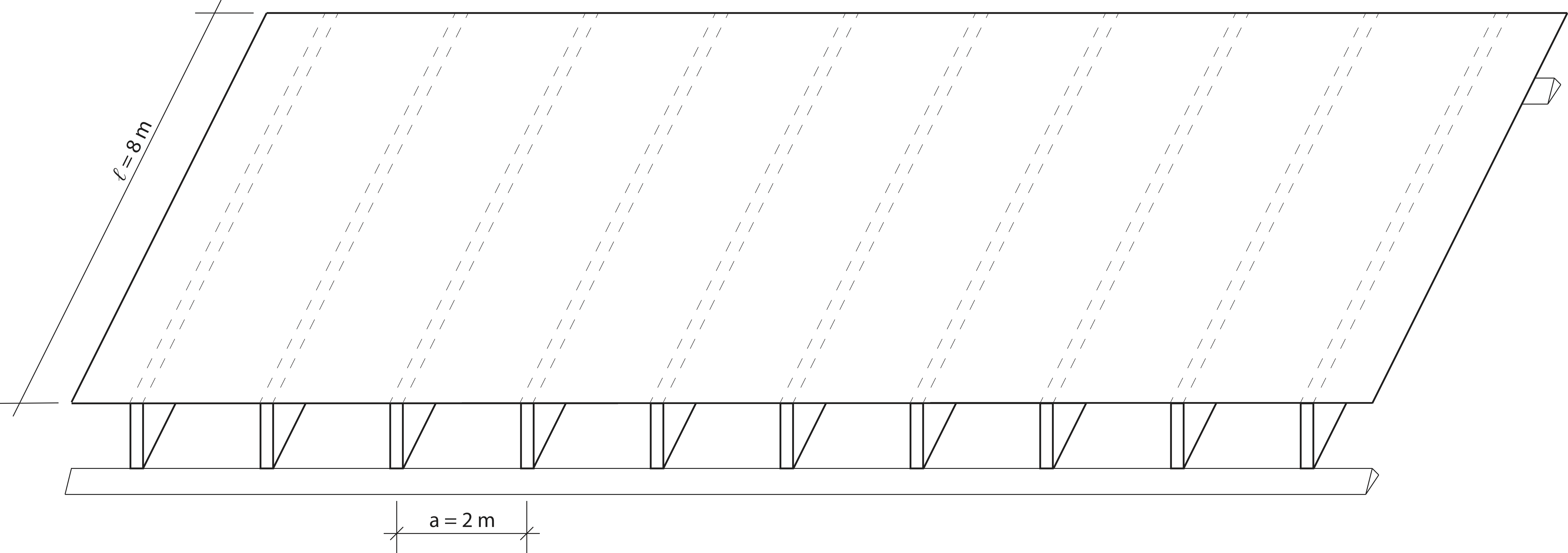
2. Conceptual design: The next logical step is the development of a principal load bearing concept of a flat roof. With the dimensions specified above a possible structural concept would be an assembly of timber beams arranged in parallel, as illustrated in Figure 7. These parallel beams (called secondary beams), are supported by larger edge beams (called primary beams).
Figure 7: Structural concept of a flat roof assembled from timber beams.

The load bearing behaviour of this concept is that the load on the roof is transferred from the roof cladding (not visible in Figure 7) to the secondary beams, which then carry the load to the primary beams through beam action, as illustrated in the next figure. We will now concentrate on the assessment of the secondary beams. The load bearing capacity of the system of secondary beams is now determined by:
- The material strength of the timber
- The distance between the secondary beams (this is decisive for how much load each beam receives), and,
- The cross section dimension of the secondary beams, i.e. the height \( h \) and the width \( b \) of a beam with rectangular cross section.
Figure 8: The flat roof as a system of beams.
3. Simplifications and assumptions: Compared to other structures, the flat roof structure is relative simple, however, a realistic 1:1 mechanical representation of this system would be cumbersome already as we would have to represent:
- How is the snow spatially distributed on the roof?
- How is the load distributed among the beams? (it obviously depends on the stiffness of the different beams and the behaviour of the edge beams at the supports, the load bearing behaviour of the columns, the roof cladding that rest on the beams etc.)
- etc.
A realistic representation of structural systems is in general rather difficult, and an important step in a structural engineering project is the identification of reasonable assumptions and simplifications. In this example, it seems reasonable to assume the following:
- The (snow-) load is uniformly distributed on the roof surface,
- The beams share the load in equal proportions,
- The transversal support beams and the columns are considered stiff.
Figure 9: The snow load is uniformly distributed, the system of beams can be decomposed to similar simple supported beams.

Figure 10

4. Mechanical Assessment: The load bearing behaviour has to be assessed. In this example we concentrate on the safety of the roof (it shall not fail) and therefore we have to assess the ultimate load bearing capacity and compare it with the load the structure is exposed to.
Bending capacity of an elastic rectangular cross section:
In order to evaluate the maximum moment load bearing behaviour of a rectangular cross section we evaluate the maximum inner moment that is dependent on the maximum stress \( \sigma_{max,timber} \) of the timber material:
Figure 11: Inner Moment: Maximum moment capacity, with \( b \) and \( h \) being the width and height of the rectangular cross section.

Moment effect of the load: The system is a simple supported beam with uniform distributed load.
Figure 12: Outer Moment: The moment distribution alongside the beam can be expressed, i.e. as a function of \( x \).

The maximum moment is found at \( x=l/2 \):
$$ \begin{equation} M_{load,max}=M_{load}\left(x=\frac{l}{2}\right)=\frac{q_s l^2}{8} \label{eq:loaMmax} \end{equation} $$Accordingly, the beam would not fail if the resistance is larger than the effect of the load, i.e. the comparison of the moments reads:
$$ \begin{equation} \frac{q_s l^2}{8}=M_{load,max} < M_{resistance}=\frac{bh^2}{6}\sigma_{max,timber} \label{eq:deq1} \end{equation} $$Equation \eqref{eq:deq1} is generally referred to as design equation. It contains design variables that are the variables that can be chosen / controlled during design. In the present example it would be the width \( b \) and the height \( h \) of the cross section that might be chosen freely and this choice is called structural design. The span of the beam \( l \) is determined by the requirements for space (the client required a roof of specified dimensions, here the area to be sheltered is 20 x 8 meters, so \( l \) would be 8 meters) and the load \( q_s=a*s \) (\( a=2\:m \)) and the material strength \( \sigma_{max,timber} \) are variables that have to be quantified.
For given \( b= \) 300 mm the required \( h \) is plotted as a function of the snow load \( s \) and the material strength \( \sigma_{max,timber} \):
Figure 13: Functional relationship between snow load \( s \), timber strength \( \sigma_{max,timber} \) and the required height of the beam. (for \( a=2\:m \), \( l=8\:m \), \( b=0.3\:m \))

But how do we quantify the snow load and the timber strength?
Snow load
The relevant snow load for design is the maximum snow load in the intended service period of the structure. A typical time duration for buildings is 50 year, i.e. we are interested in the extrem snow load event in a period of 50 years. As the snow load will vary over time and future snow loads cannot be predicted with certainty, the snow load - as other types of loading - has to be represented with random variables that are specified based on measurement data.
The snow load is also very much dependent on the geographical location and on the altitude of the construction site. In Figure (14) the geographical distribution of the snow load with an average return period of 50 years is illustrated. This value is also referred to as the characteristic value of the snow load. This map is part of the national annex of Eurocode EN1991 for snow loads.
Figure 14: The characteristic snow load on the ground in Norway.
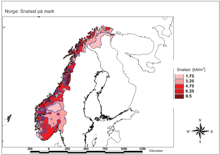
From the map and corresponding tables a value of \( s_k=3.25 kN/m^2 \) for Trondheim could be identified.
Timber strength
The properties of solid timber are characterised as the load bearing performance properties of solid timber components exposed to different loading modes, see Figure (15). Accordingly, the strength and stiffness related properties of structural timber are communicated as the properties measured in standardised experiments i.e. with standardised dimensions, loading modes and duration, and surrounding climate.
Figure 15: Different loading modes on structural timber that are generally referred to as material properties.

Timber material for structural purpose is generally associated to a certain grade or strength class. In Europe timber strength classes are defined as sub-populations with expected values for the 5th-percentile of the bending strength and timber density, and expected values for the mean value of the bending stiffness. Properties corresponding to other loading modes per timber strength class are also given, see Figure (16). (The mentioned material properties are defined as properties of standard test specimen according to corresponding test standards).
Figure 16: Different loading modes on structural timber that are generally referred to as material properties.
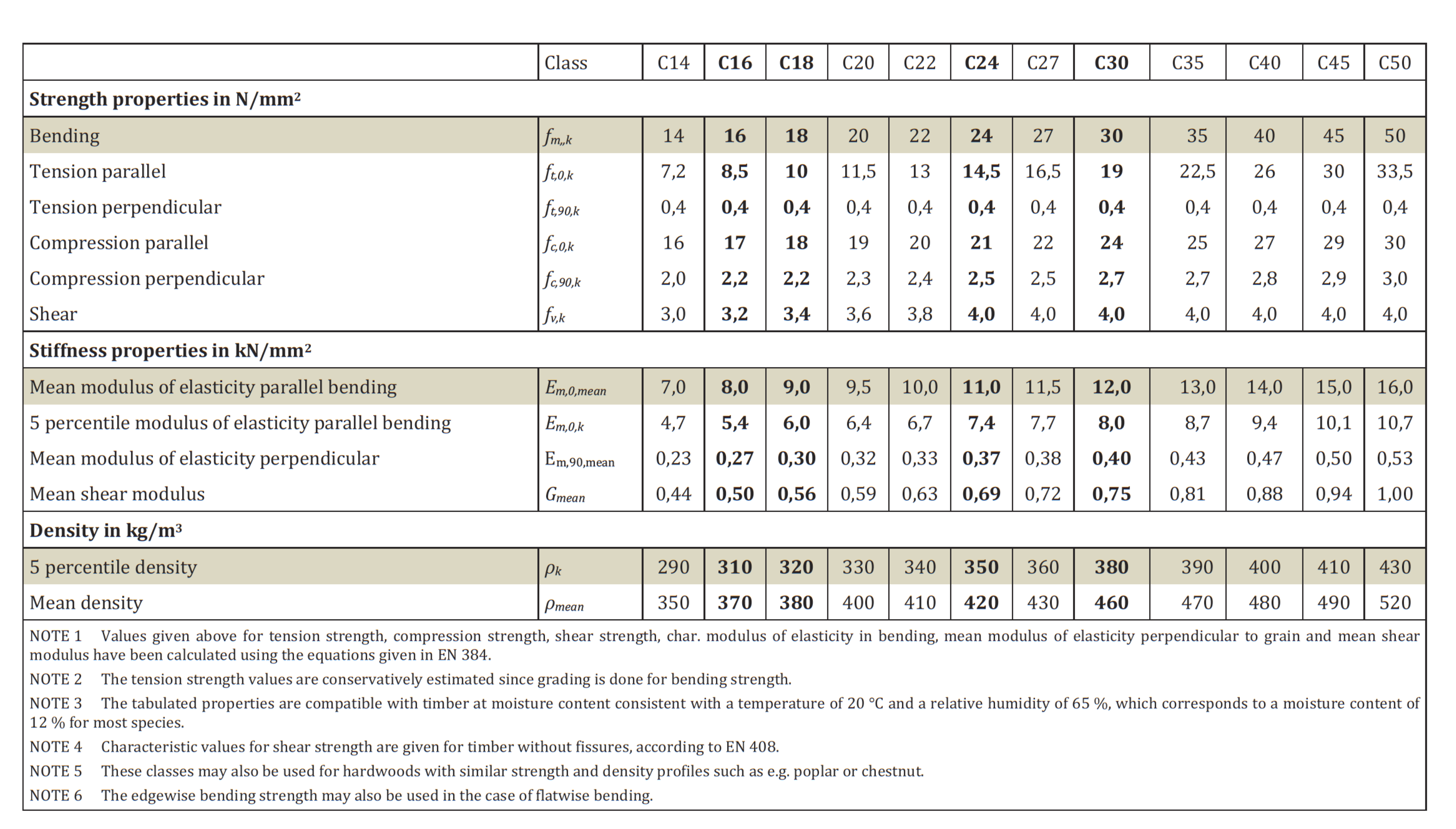
For the very typical strength class C24 the bending strength of \( \sigma_{max,timber}=f_{m,k}= \) 24 MPa can be specified.
Probability Distribution?
We can guess it already: The material strength and the snow load are uncertain - i.e. they cannot be specified unambiguously. What we can specify is with which probability a specific value is exceeded or not. The function that is representing this probability is called Probability Distribution Function. The Probability Distribution Function is defined over the possible domain of the variable \( X \) (this is a random variable and this is indicated by a capital letter) and attains values \( x \) (or realisations - indicated by a small letter). Figure (17) shows a probability distribution function \( F_X(x) \) and so-called fractile values. The 5%-fractile value is the value with a non-exceedence probability of 0.05 or 5%, i.e. \( F_X(x)=Pr(X < x)=0.05 \). The characteristic value of the snow load is defined as the 98%-fractile of distribution of the yearly extreme values.
It can be seen that the characteristic values of the material strength and the load are chosen as a lower and upper fractile correspondingly. But is this a sufficiently safe assumption?
Figure 17: Probability distribution function and fractile values.

We will follow up on this question during this course - but first we will start with the introduction of principle structural systems and concepts in the next lecture.
Challenge yourself:
- Try to produce a figure like Figure 13 with the software of your preference (e.g. Excel, Python (recommended), Mathlab, etc.).
- How deep is freshly fallen snow that induces a load of \( 3.25\:kN/m^2 \)? Make a informed guess!
- Develop Equation \eqref{eq:inM} considering simple geometry.
- Develop Equation \eqref{eq:loaMmax} considering the principle of force equilibrium.
Lecture 2 - Understanding structures
The learning goal of today is:
- gain overview about principle structural elements and the functionality
- introduce typical structural systems
- link to structural mechanics
- qualitative load effects on structures
Reading / Homework:
- Reading the lecture notes distributed on BlackBoard
- Rework the examples from the lecture
- Per Kr. Larsen - Konstruksjonsteknikk: Chapter 3
Structures
A structure is an arrangement and organization of interrelated elements in a material object or system, or the object or system so organized.— Oxford English Dictionary (Online ed.). Retrieved 1 October 2015.
In the context of the build environment, structures are understood as an assembly of components or elements for the purpose of load bearing. However, the primary purpose for load bearing, and therefore for structures is to support societal activities, i.e. provide for shelter, transport, energy production etc.
Depending on the load bearing purpose, some principle structural components with advantagerous and specialized load bearing behaviour have been developed and a summary is found next.
Principle structural components
Principle structural components are introduced and their principle load bearing behaviour is explained. Examples for implementation with different materials are given.
Rod/Bar
(Stav)The probably simplest structural element is the rod or bar. It is characterised by its relative slenderness (slankhet), i.e. one dimension is significantly bigger than the remaining ones. As due to this slenderness the rod works best if it is loaded axially in tension. Rods are often made of steel but also rods in timber or reinforced concrete can be found.
Figure 18
Load bearing behaviour:
Figure 19: Principle sketch of a rod with cross section \( A \) and ultimate tension strength \( f \). The rod is loaded by the force \( F \).
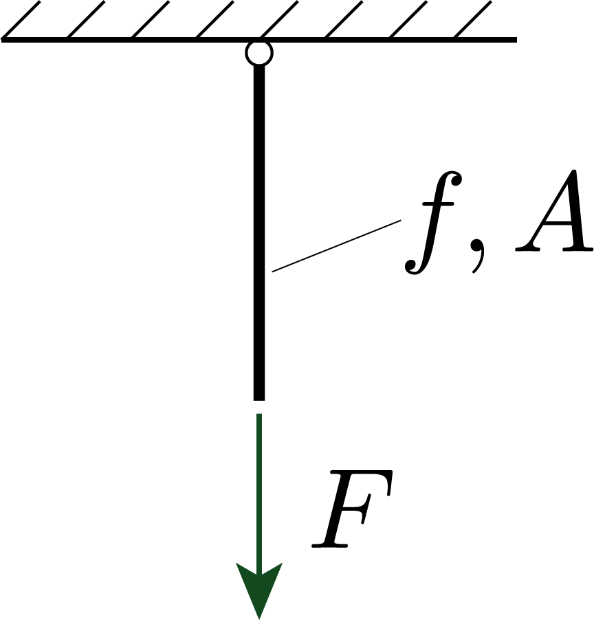
The load bearing resitance \( R \) in \( [N] \) of a rod can be calculated as
$$ \begin{equation} R=f \cdot A \label{} \end{equation} $$where \( f \) is the ultimate material strength in \( [N/mm^2] \) and \( A \) is the cross section area in \( [mm^2] \).
Example Rod 1:
We want to support a load \( F=1 \; MN \) (mega newton) by a steel rod. The steel is a type of high strength steel and has a ultimate resistance of \( f=600 \; N/mm^2 \). The rod is supposed to have a circular cross section. What is the diameter to choose?
Solution:
- We want to prevent rupture or failure so we should choose the cross section \( A \) such that:
or
$$ \begin{equation} A > R = \frac{F}{f} = \frac{10^6 \; [N]}{600 \; [N/mm^2]} =1666,67 \; mm^2 \label{} \end{equation} $$- With a circular cross section this corresponds to \( d=46.1 \; mm \) (\( A=d^2 \frac{\pi}{4} \)).
Picture the orders of magnitude here: How many tonns \( [t] \) is \( =1 \; MN \)? How many Tesla model X does this correspond to? Draw a circle of 46 mm and wonder!
(End of example)Challenge yourself:
We want to calculate the maximum lenght a unloaded rod can take. In the example above we ignored the self weight of the rod as it is order of magnitudes smaller than the external loads. In this example we look only at the self weight and we want to find out at which length a hanging rod would fail.
Principle solution: Again we assess the situation where the load bearing resistance is equal to the loading. In the case of loading by self weight we might write:
$$ \begin{equation} R = f \cdot A = \gamma \cdot A \cdot l_{max} \label{} \end{equation} $$where \( \gamma \) is the material specific weight and \( l_{max} \) is the lenght of the rod.
We see that \( A \) canceles out and the maximum lenght \( l_{max} \) only on two material properties, i.e.
$$ \begin{equation} l_{max}=\frac{f}{\gamma} \label{} \end{equation} $$The solution is as expected dependent on the ratio between strenght and specific weight.
In the following table some values for some typical building materials are given. Graphen and ice are only added for interest, they are less relevant for usual structural applications.
| Material | Density \( \rho \), \( [kg/m^3] \) | Specific Weight \( \gamma \), \( [kN/m^3] \) | Strength (e.g.) \( f \), \( [N/mm^2] \) |
| Steel | 7850 | 78.5 | 500 |
| Concrete | 2300 | 23 | 2 |
| Timber | 500 | 5 | 24 |
| Graphene | 2270 | 2.27 | 130000 |
| Ice | 910 | 9.1 | 1 |
Challenge: Calculate the maximum hanging lenght yourself!! How would you optimize the shape of the rods in order to reach even larger values for the length??
(End of example)Column
(Søyle)Figure 20
A column is a structural element that is intended to transfer loads by acting mainly in compression. For example, a column might transfer loads from a beam or from a slap or roof to a foundation.
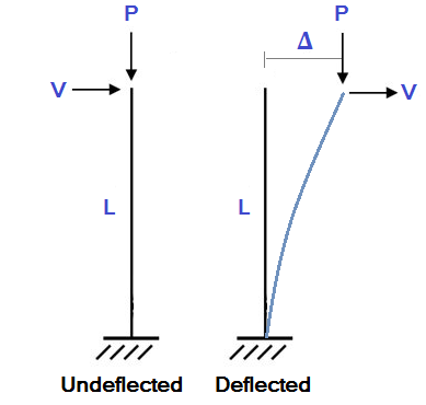
Similar to rods, columns are slender in general, however, the load bearing capacity is decreased non-linearly with increased slenderness. This effect can be illustrated by the following sketch. The moment in the support is \( M=V \cdot L \) considering the undeflected state. However, due to the moment, the column would bend. The moment is actually increasing to \( M=V \cdot L + P \cdot \Delta \). The load effect (the moment) is progressively increasing with increasing \( P \). This is referred to as the \( P-\Delta \) effect. The load effect becomes also dependent on the lateral stiffness, i.e. on the slenderness of the column.
Figure 21
A informative video is showing a laboratory test of a slender column. It is provided by Imperial College, London:
The slenderness (slankhet) is defined as
$$ \begin{equation} \lambda=\frac{L_k}{i} \text{ with } i=\sqrt{I/A} \label{} \end{equation} $$where \( L_k \) is the buckling length (knekklengde), I is the moment of inertia, A is the cross section area.
Figure 22: Columns with different boundary conditions have different bucklinglength \( L_k \)
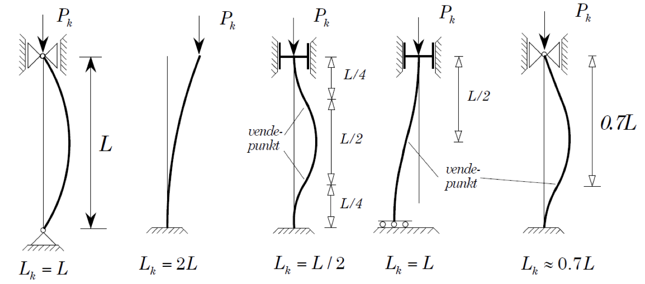
It is said the \( P-\Delta \) effect is more pronounced for low slenderness. For a given buckling length \( L_k \) the slenderness is decreasing when \( I \) is getting larger in relation to \( A \). Cross section geometries of columns are thus chosen to obtain a large value for \( I/A \).
Challenge yourself:
- Which cross section geometries are most suited for columns?
- Which are not so good?
- Explain your choices!
Figure 23
Beam
(Bjelke)Figure 24
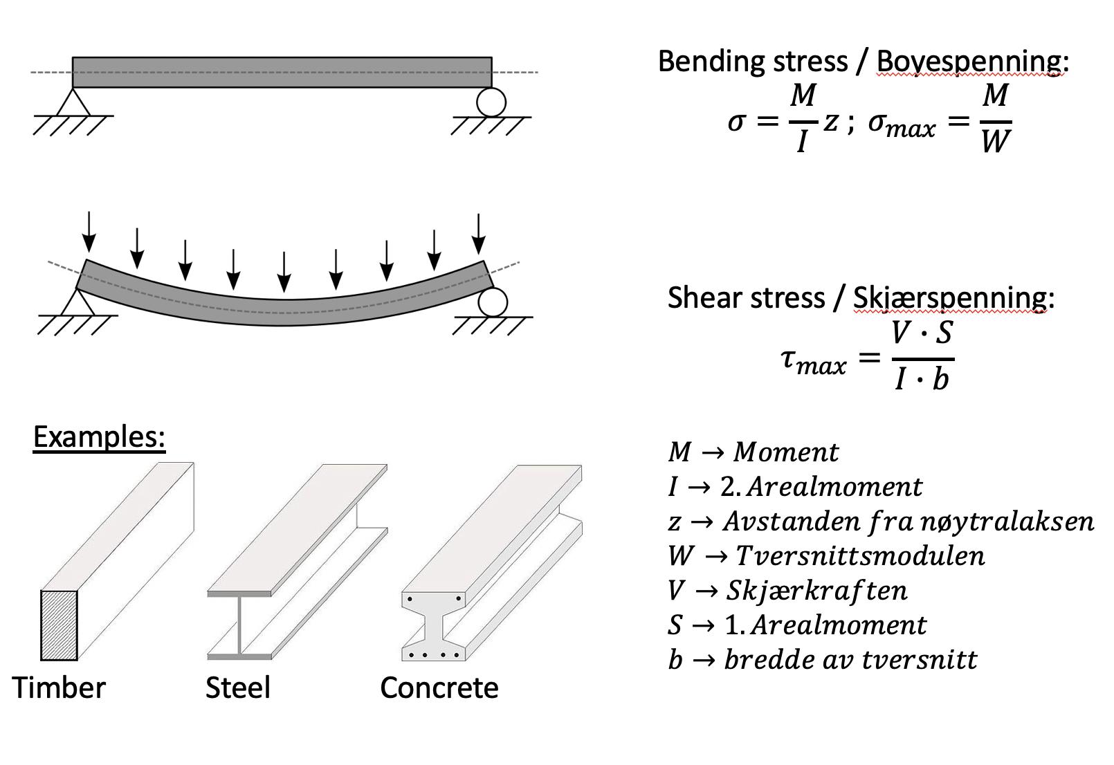
A beam is a structural element that primarily resists loads applied laterally to the beam's axis which result in reaction forces at the beam's support points. Shear forces, bending moments and possibly normal forces within the beam, are the corresponding load effects.
Figure 25: Principle sketch of a simple supported beam. The bending and shear stress is evaluated based on the moment and shear-force correspondingly. Example beam cross sections for different structural materials are given.
For more insight to the basic principles of beams in bending provided by Dr. G. Wayne Brodland from University of Waterloo:
In a structural system beams transfer loads imposed along their length to their end points where the loads are transferred to other beams, walls, columns, etc.
Beams may be manufactured from timber, steel, or concrete or they may be composite constructions.
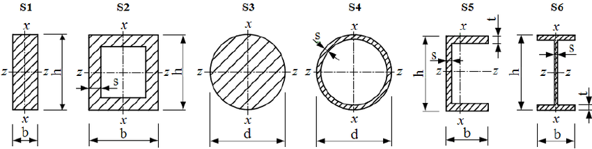
A wide variety of cross section shapes are commonly available, including; square, rectangular, circular, I-shaped, T-shaped, H-shaped, C-shaped, tubular, etc. The cross section shapes are chosen such that they display a large section modulus.
Beams may be straight, curved or tapered.
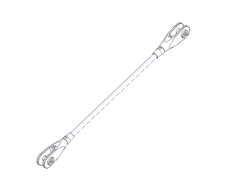
Cables
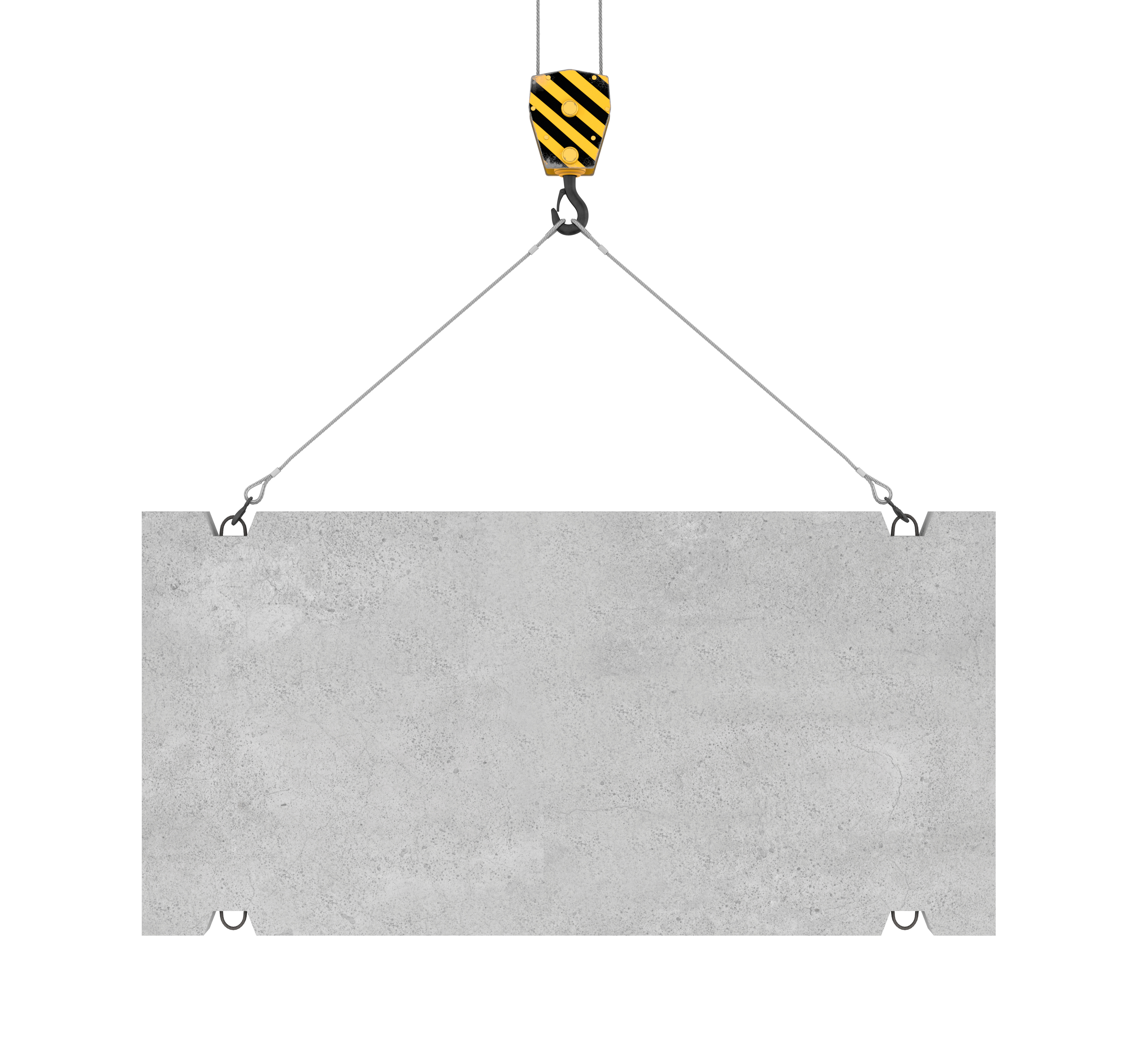
Figure 26

As rods, cables are intended to carry tension forces, but in addition cables have a relative high flexibility in bending and shear such that they can be used very effectively for large and light structures. Cable structures include the suspension bridge, the cable-stayed roof, and the so-called bicycle-wheel roof. Cables for structural purpose are mainly made of high strength steel and the tension capacity is very high - so high that it is always a technical challenge to anker these high forces at the end of the cables. When lateral loads are introduced, typically by clamps (see above), the shape of the cable adapts. This principle is well utilised e.g. for suspension bridges where huge suspension cables carry impressively large spans.
Figure 27: An almost iconic cable structure is the golden gate bridge in San Fransisco, US. The suspension cable is guided over two 227m high towers and supports an overall span (shore to shore) of 2737m, tower distance is 1280m. Note that the cables are anchored in the ground by huge foundation blocks that are partly hidden behind the flowers on the left side of the picture.

For suspension bridges there is an interesting relationship between tower hight and cable force as nicely illustrated with the example of the Golden Gate bridge.
For more insight to the basic principles of suspension bridges, watch this interesting video provided by Dr. G. Wayne Brodland from University of Waterloo:
A free hanging cable (or chain) has to carry its own self weight and its shape is following the so called Canetary line that is mathematical described by
$$ \begin{equation} z=f(x)=a \cdot cosh\left(\frac{x}{a}\right). \label{} \end{equation} $$A cable that is considered weightless but is carring a horizontal uniform distributed load as e.g. the bridgedeck of the Golden Gate bridge is following a parabola shape, i.e.
$$ \begin{equation} z=f(x)=b\cdot x^2. \label{} \end{equation} $$Figure 28: a) The shape of a cable or chain that is only loaded with its own self weight is following a catenary line; b) the shape of a cable or chain that is only loaded with an external uniformly distributed load is following a parabola.

Figure 29: The catenary line and the parabola have very similar shapes. For large cable structures this small difference is significant and has to be considered carefully.
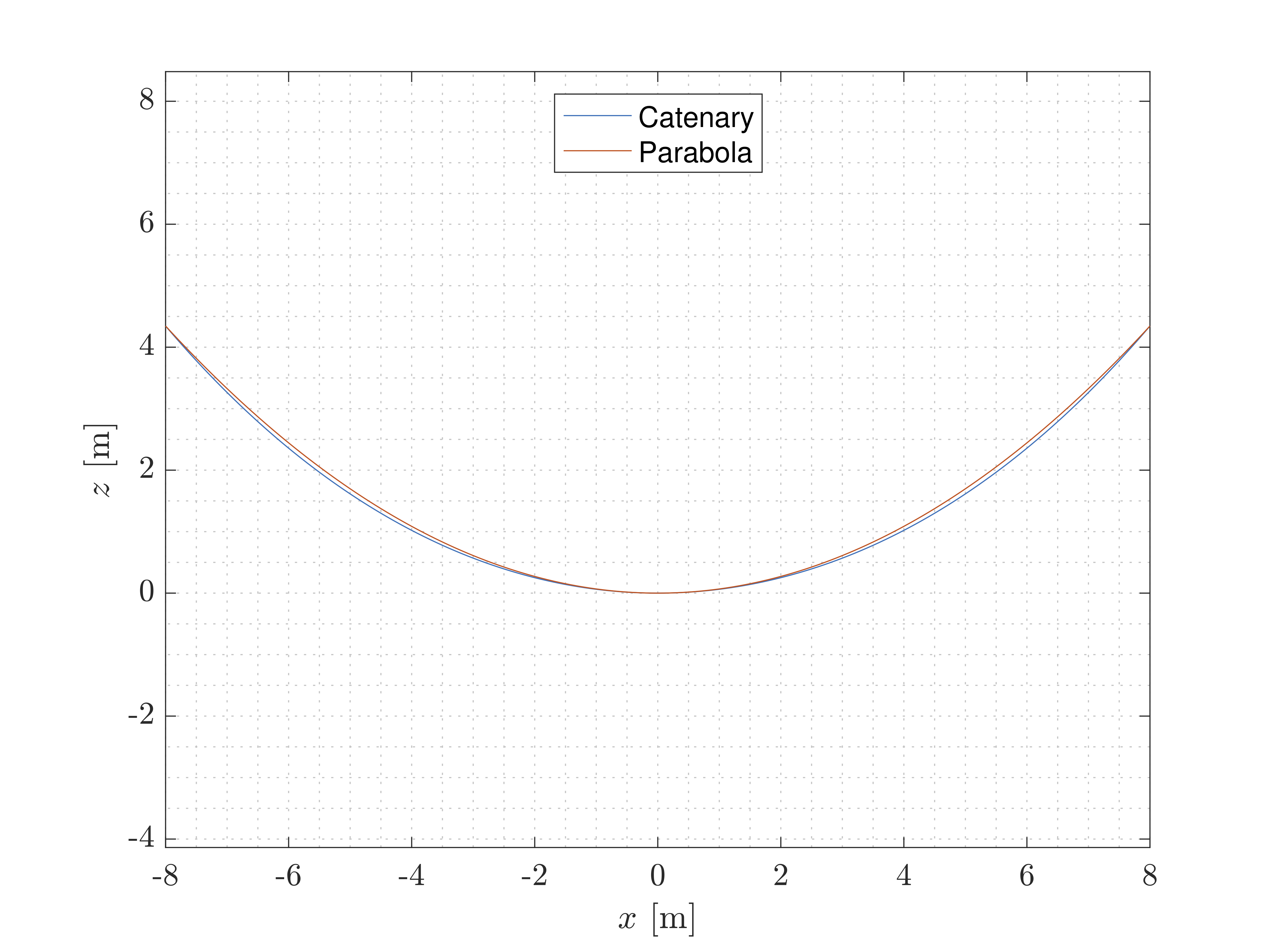
Figure 30: Cables are also used to create large spans for buildings, here the Alamodome, San Antonio, US. Note how the tension forces are anchored to the ground.

(Picture by Billy Hathorn - CC BY 3.0).
Challenge yourself:
Consider the Canetary line in Figure 27 (a). Assume that the length of the cabel is \( l=7\:m \), the distance between the supports is \( s=5\:m \) and the total mass of the cable is \( m=450\:kg \).
- What is the horizontal reaction force at the supports?
- What happens if you change \( s \)? Make a graph showing the horisontal reaction force over the distance between the supports \( s=(0,7) \) (\( s \) in the open interval between 0 and 7).
Arch
(Bue)Figure 31

An arch is a vertical curved structure that spans between supports and supports its own weight and the weight above it. In an arch transversal loading is resolved mainly or entirely into compression stresses and this is often referred to as arch action. The arch action principle is illustrated in the figure - following the right shape, it is possible to create pure compression actions in the arch.
Figure 32: When an arch is very slender, the correct shape is of utmost importance. (credit)

For more insight to the basic principles of arches, watch this interesting video provided by Dr. G. Wayne Brodland from University of Waterloo:
The arch action effect did facilitate create large spans by using of simple building materials as rock and bricks that only work in compression. This is the reason that arches are a dominant building principle for creating spans in ancient construction.
Figure 33: How many arches do you find in Nidarosdomen? - and how many beams...?

The principle of arch action is also utilised to create span in two dimensions and this is called vault (hvelv).
Figure 34: A nice example of a vault is found in Bristol, England.

Figure 35: The arch action principle is the predominant structural principle for ancient bridges and aqueducts, here the Pont du Gard in France.

The arch action has also a "side effect" that is important to consider. As the forces on the arch are transfered to the ground, a horizontal force develops, that, if not restrained will push the arch outward at the base. This is called thrust. As the rise, or height of the arch decreases, the outward thrust increases (note that this is one of the reasons for the several "storeys" of the Pont du Gard, see picture above). The thrust is restrained e.g. by internal ties or external bracing, such as abutments.
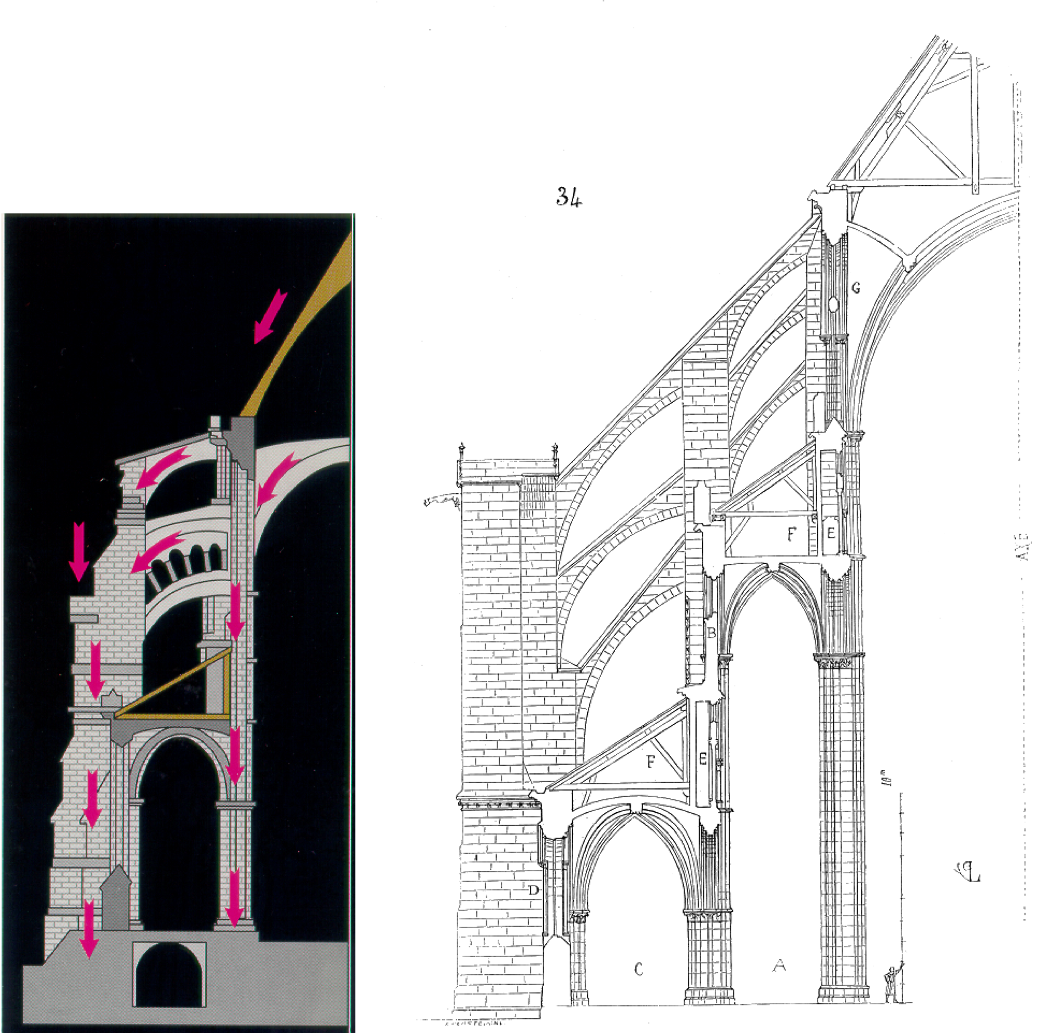
Figure 36: The principle architectural layout of ancient cathedrals is dominated by the need of restraining horizontal forces from arches and vaults. This is e.g. the reason for the classical arrangement of one main aisle and two side aisles as well as external abutments. Here, the external abutments can be clearly identified.

Figure 37: The external abutments transfer horizontal loads into the ground.
For more insight on how cathedrals work, watch this interesting video provided by Dr. G. Wayne Brodland from University of Waterloo:
Dome
(Kuppel)A dome is point symmetric structure, and the dome action is comparable to the arch action, it transfers the loading outwards keeping the internal forces mainly in compression. The dome can be self-restrained if tension force can be carried tangentially at the lower edge of the dome, i.e. the edge is usually reinforced by a so called ring beam.
Figure 38: This is not a Unidentified Flying Object (UFO) - for most structural engineers this is THE highlight of the visit in Rome, Italy. It is the Patheon - and it is a dome.

Figure 39: The Pantheon has a inner diameter of 42m and is made of concrete. The construction was finalised around the year 125 AD. (Note that concrete was forgotten in the middle-age and "reinvented" in the mid-18th century.)

If the geometry is getting more free but the principle of transferring lateral loads mainly by compression action the structure is called shell structure. Thin freeform structures mainly acting in tension are called membran structures. Both structures make use of so-called membran action created by the interaction of in-plane forces.
Figure 40: The Sydney Opera has a shell structure as a roof.

For more insight on how domes work, watch this interesting video provided by Dr. G. Wayne Brodland from University of Waterloo. This video is also very useful if you want to construct an igloo.
Challenge yourself:
Figure 41

When the winter came back: Find some friends, go to the forest and build and igloo. Send pictures of your result to jochen.kohler@ntnu.no.
Hints:
- Dress appropriately. It might be cold.
- Take some precautions, the igloo might collapse during construction.
- Find a nice and flat area with a good supply of snow.
- Snow that has been carried by wind has very good structural properties. You should find plenty of that kind right now.
- A recommended toolset is a spade and a large wood saw (håndsag).
Truss
(Fagverk)Figure 42

A very important structural type is the truss, which is basically a plane or three-dimensional system of triangular compositions of rods.
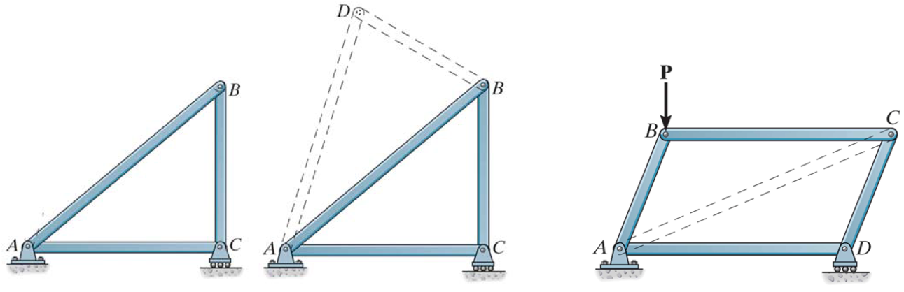
Figure 43: In a truss, rods are connected with hinges. The triangular is the smalles stable element of a truss.
A truss has many advantages; it is light and transfers loads very effectively alongside its rod elements. The overall shape of trusses can be always related to principle building elements like beams (see the truss bridge above), columns, arches, domes.
Figure 44: A truss as a column: Radio masts are impressive structures. The highest ever build (in 1971) was the Warsaw radio mast and with a height of 646m(!) it was the highest structure at the time. It collapsed in 1991 due to lack of proper structural maintenance.
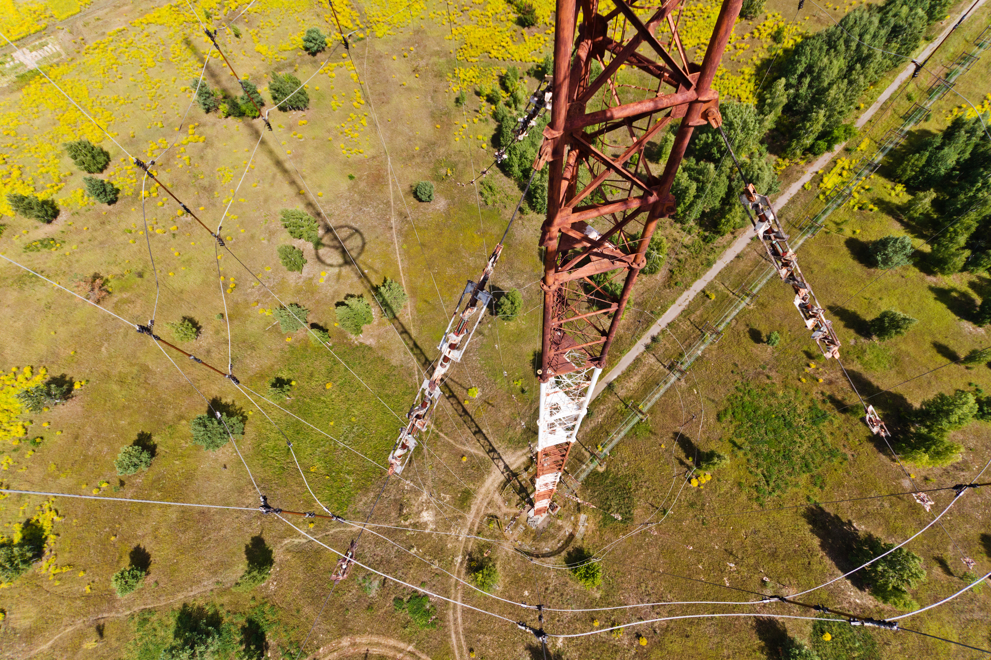
Figure 45: A truss as a arch: The Harbour Bridge in Sydney build in 1931 with a span of 503m. The main load bearing part consists of a steel truss with the shape of an arch (and thereby utilising the corresponding structural benefits). Notice the group of people on the top of the arch (just zoom a bit in).

Figure 46: A truss as a dome: This elegant structure (93m diameter, 31m height) is used for the storage of 90 000 tonns de-icing salt in Switzerland. The truss is made of timber that is also well suited to cope with the aggressive environment created by the salt - much better than steel and reinforced concrete.

Another facinating dome / truss structure is the Sports Hub in Singapore.
Figure 47: Here we see a truss in a rather untraditional application. Which truss elements are in tension - which in compression?
There is also a very didactic video on the web. As it is associated with comercial clips I only add it as an external LINK. It is suggested to ignore the commercials!
Slabs and Plates
(Skive / Plate)Figure 48
A slab is a plane element where one dimension is significantly smaller than the other two. It is used either upright (as wall) or flat (as ceiling or floor). A wall slab is mainly loaded in plane in shear and compression. A horizontal slab is loaded laterally and often also in shear.
Figure 49: The sketch illustrates a system of columns and slabs. The latter are very important for the overall stability of the structure – the slabs work in in-plane shear to stabilise the structure.
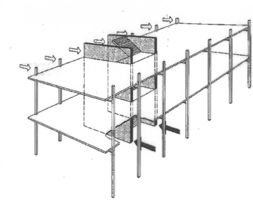
Figure 50: Columns and slabs. The slender columns transfer only vertical compressions forces introduced by the slab/plate. The vertical slab/wall is transferring compression forces. Both slabs are very important for the overall stability of the structure as they also transfer shear forces at the occasion of horizontal loading (e.g. due to wind, earthquake, geometrical imperfection).

A very nice model for exploring the bending behaviour of laterally loaded plates is introduced by Dr. G. Wayne Brodland from University of Waterloo.
Connections and supports
Figure 51
Structural components are assembled to structural systems in order to create volume and space. Thereby, loads have to be transfered to the supports and finally to the ground via several connections between the components. It is in general distinguished between different principle types of connections and supports all dependent on what kind of action they can transfer.
Figure 52: This nice illustration is taken from Kolbein Bell/IKT/NTNU. It shows the most important structural supports being the fixed- or restrained support (fast inspenning), the pinned support and the sliding support (rullelager). The corresponding restrains and reaction forces are also indicated in the figure.
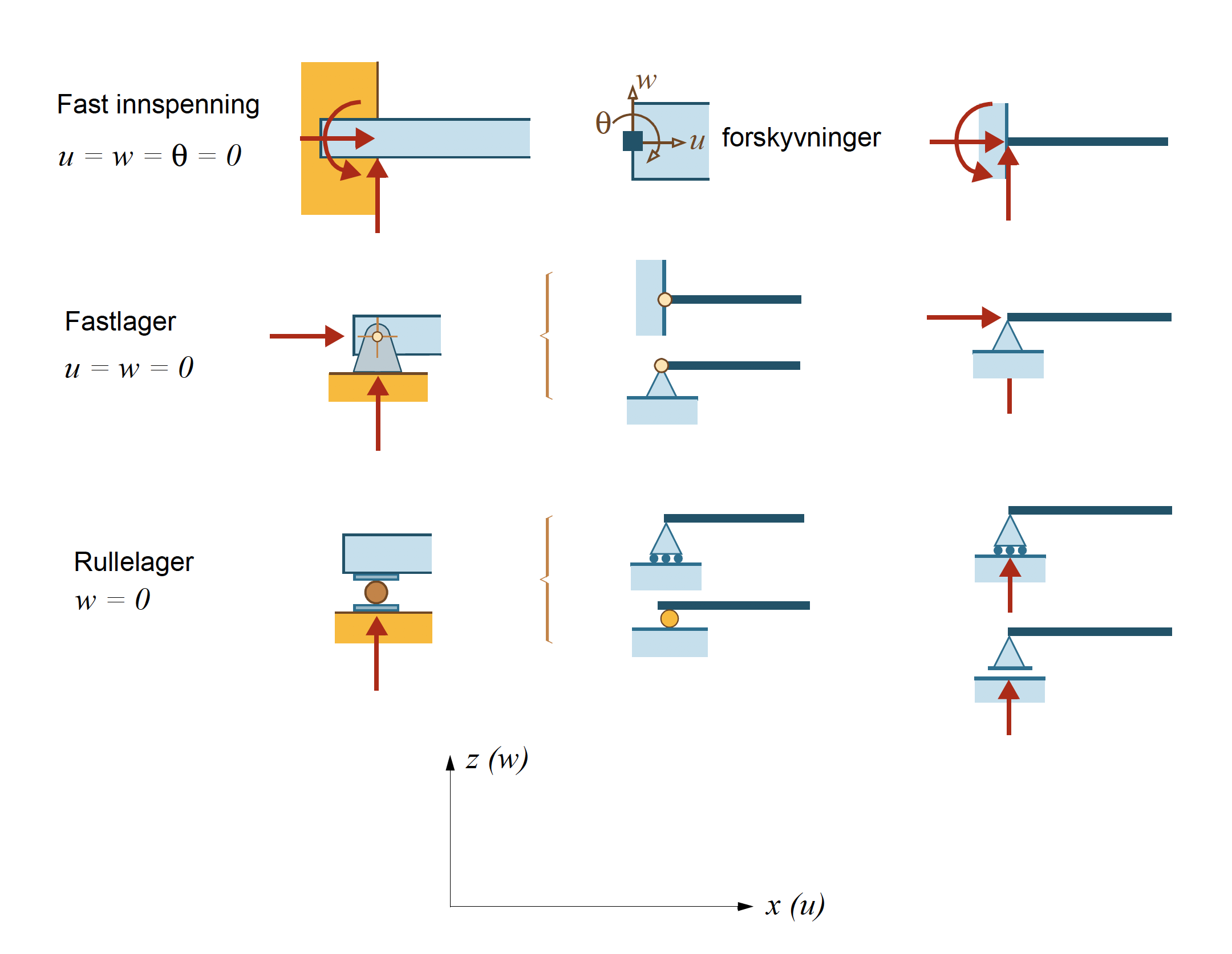
Figure 53: For joints it is most importantly distinguished between hinged and continuous connection whereas the former does not take any moments, i.e. the moments at the hinges are equal to zero by definition. Illustration taken from Kolbein Bell/IKT/NTNU.
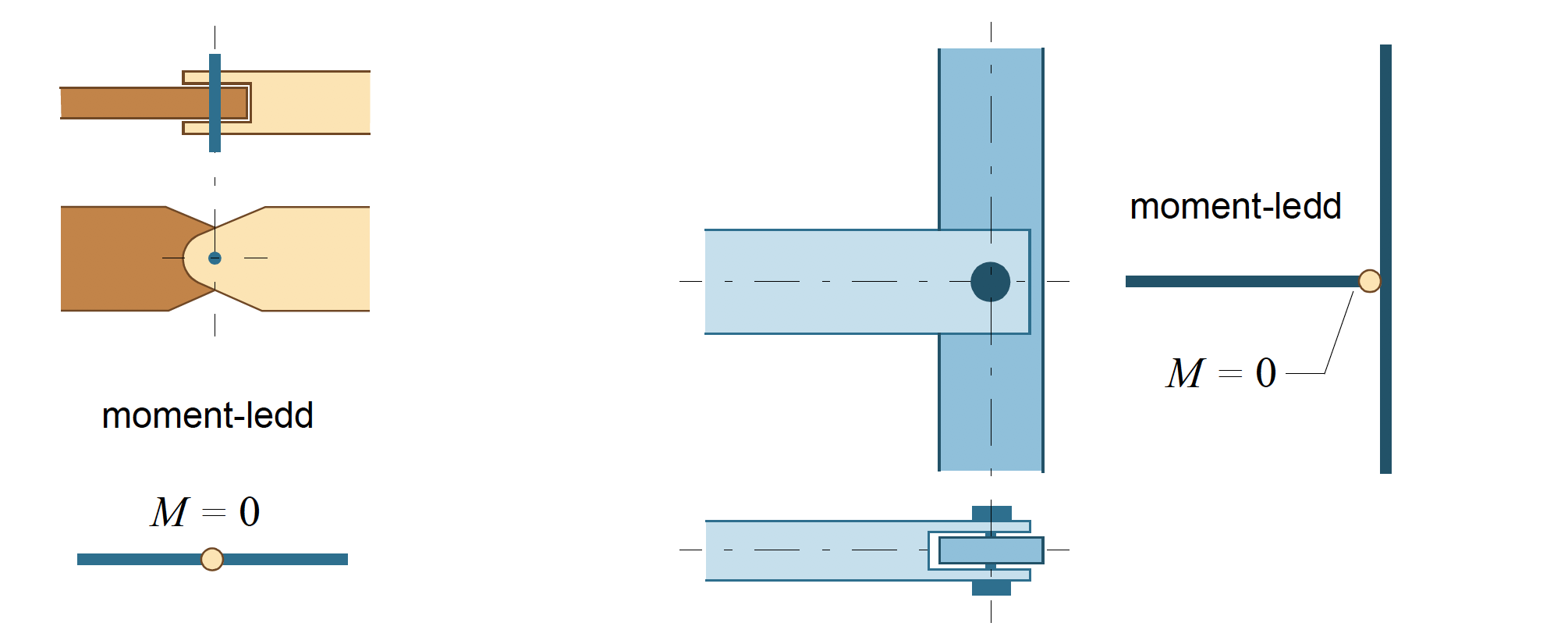
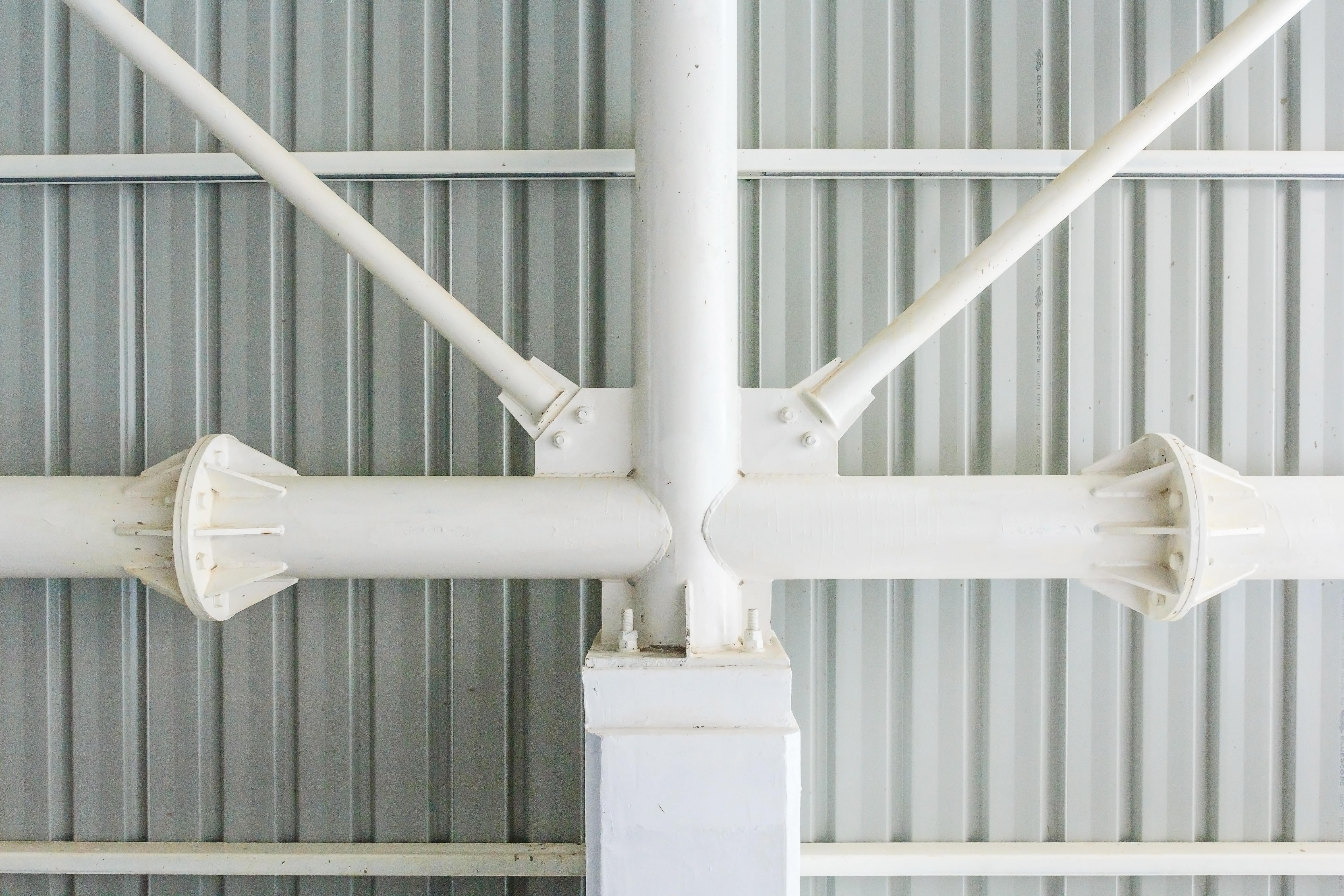
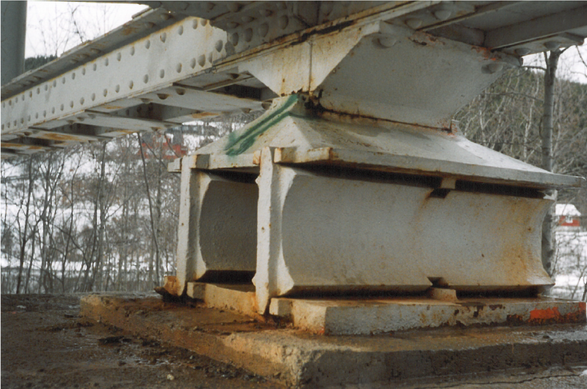
These principal types of connections and supports are used in mechanical computations. It is interesting and sometimes surprising how these principle types look in real structures.
Figure 54: What kind of support is this?
Foundations
Figure 55

Foundations are the very important prolongation of structural systems towards the ground. The further discussions of foundations is outside of the scope of this lecture and it is referred to the corresponding lectures in geotechnics for obtaining more insight.
Further recommended didactive videos:
Challenge yourself:
Wait for better weather and then go for "Structure-Safari" (ideally as a group).
Hints:
- Dress appropriately. The weather might turn bad.
- Take a camera and something to make notes.
- Look for basic structural elements in buildings and bridges.
- The "Realfagbygget" at Gløshaugen is actually a good start. But there are much more interesting buildings and other structures in Trondheim. Construction sites are also very interesting to observe.
- Make pictures and notes. Which type of elements do you see? What kind of loads do they support? Where is the highest load effect?
- Make a small report. And if you want share it with me.
Lecture 3 - Principle Load Effects in Structures (Part 1)
The learning goal of today is:
- be able to qualify priciple load effects in structures
- understand vertical and horizontal load bearing in buildings
- excersises on structural load effects
Reading / Homework:
- Compendium: Lecture 4 (and 1 + 2 + 3 if not done yet)
- Per Kr. Larsen - Konstruksjonsteknikk: Chapters 3 + 4
- 1. comulsory excersise
Principle load bearing behaviour of structural elements and systems
Figure 56
Basic Principles
The load bearing behaviour of structural elements and systems is dependent on:
- The geometrical proportions of the structure
- The location and the restraint of supports and connections
- The magnitude and spatial distribution of loads
- The stiffness of the structure
It is important to note that the first two aspects can be controlled pretty well by structural design. The magnitude and spatial distribution of loads, however, is normally not known exactly in advance and it might also change over time. This means that any assumption is associated with large uncertainties. The uncertainties about the time variability are normally explicitly taken into account and we will discuss this later in the lecture in more detail. The uncertainties about the spatial distribution of loads are often accommodated by conservative simplifications, i.e. a worst case placement of the loads and this introduces a large bias into the mechanical assessment.
Load bearing behaviour is assessed in terms of the structural response to loads and the response can be fundamentally expressed in stress and strain. It is in general practically beneficial to introduce an intermediate level that is called load effects and that can be axial forces, shear forces, moments and deflections.
The analysis of the load bearing behaviour can become complex and demanding especially for complex structures and if a high accuracy (a very realistic representation) is necessary/requested. More complex analysis is often performed with the aid of numerical methods and computer programs and belongs to the domain of specialised structural engineers. For simpler problems the application of some straight forward principles is generally sufficient. And even for the before mentioned more complex problems, the application of these straightforward principles is delivering important insight about the underlying load effect proportions and magnitude and should always be used for error checking of the output of the corresponding computer programmes.
The basic principles for structural analysis are:
- static equilibrium (\( \sum M=0 \), \( \sum F_z=0 \), \( \sum F_x=0 \), see sketch above)
- assumed linearity (load effect is increasing lineary with increasing load)
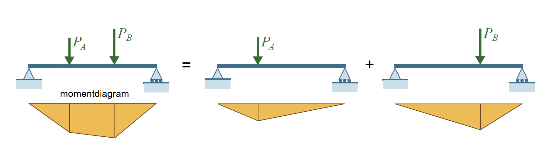
- superposition
It is important that each civil engineer has developed a basic understanding on the application of these simple principles to structures. The ability for rough assessment of the main structural functionality and the order of magnitude of forces and stresses for the purpose of quality check or conceptional design is important not only for specialised structural engineers.
For statically determined structures, the principle of Equilibrium is utilized to qualify and quantify internal and external response to forces, i.e.
- The reaction forces at the supports.
- The internal forces (and moments) at any abritary segment of the structure.
Figure 57: Reaction forces and internal forces are determined by equilibrium considerations. Illustration Kolbein Bell.
A very good video about Equilibrium is provided by Dr. G. Wayne Brodland from University of Waterloo:
Figure 58: Superposition is utilized for structuring more complex systems and load situations - here a not so complex example. Illustration Kolbein Bell.
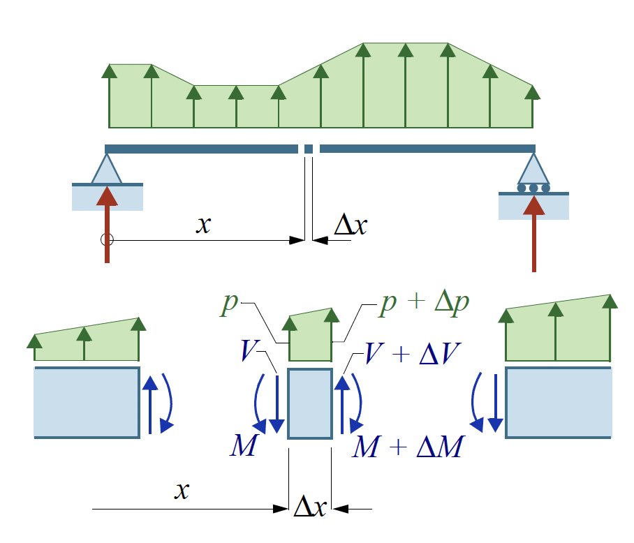
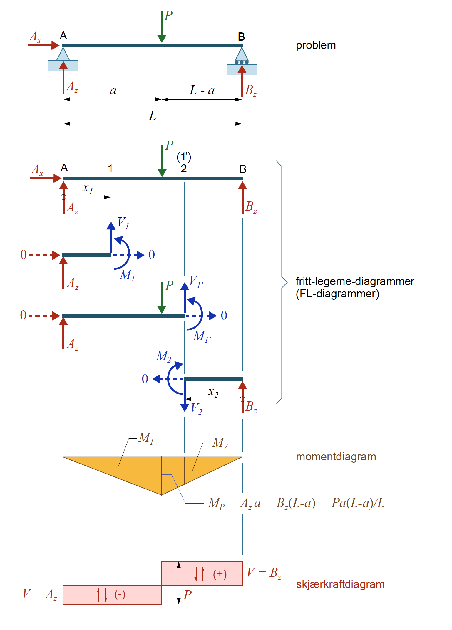
Moment- and Shear-force distribution
Figure 59: Example how the moment and shear-force distribution is obtained by equilibrium considerations. Illustration Kolbein Bell.
If systems become more complex, it might be wise to remember some basic rules:
- Sperate the structural system at possible hinges to sub-systems.
- Replace the hinges by simple supports that take vertical and horizontal forces.
- Determine the reaction forces at the sub-systems based on rigid body equilibrium.
- Remember that moments are zero at all ends and at supports that are not fixed.
- The momentline is drawn on the tension side of the beam.
- Shear-force is only changing at locations with loading or reaction forces.
- Single forces lead to blocks of uniform shear-force and triangular moment distribution.
- Uniform line loads lead to triangular shear-force and quadratic moment distribution.
- The maximum (minimum) moment is found where the shear-force is zero.
- Shear-force and normal force are swapping at rectangular frame corners.
- Moments are continuous at moment resistant frame corners.
Figure 60: Some of the rules are here nicely illustrated. Illustration Kolbein Bell.
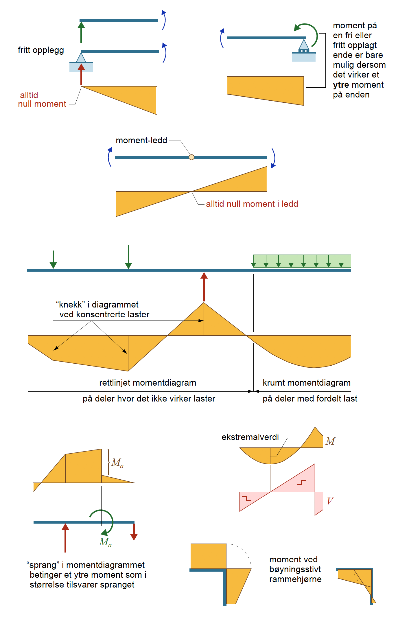
Figure 61: An example on how the support conditions change the force diagrams. Illustration Kolbein Bell.

Further Problems
Challenge yourself:
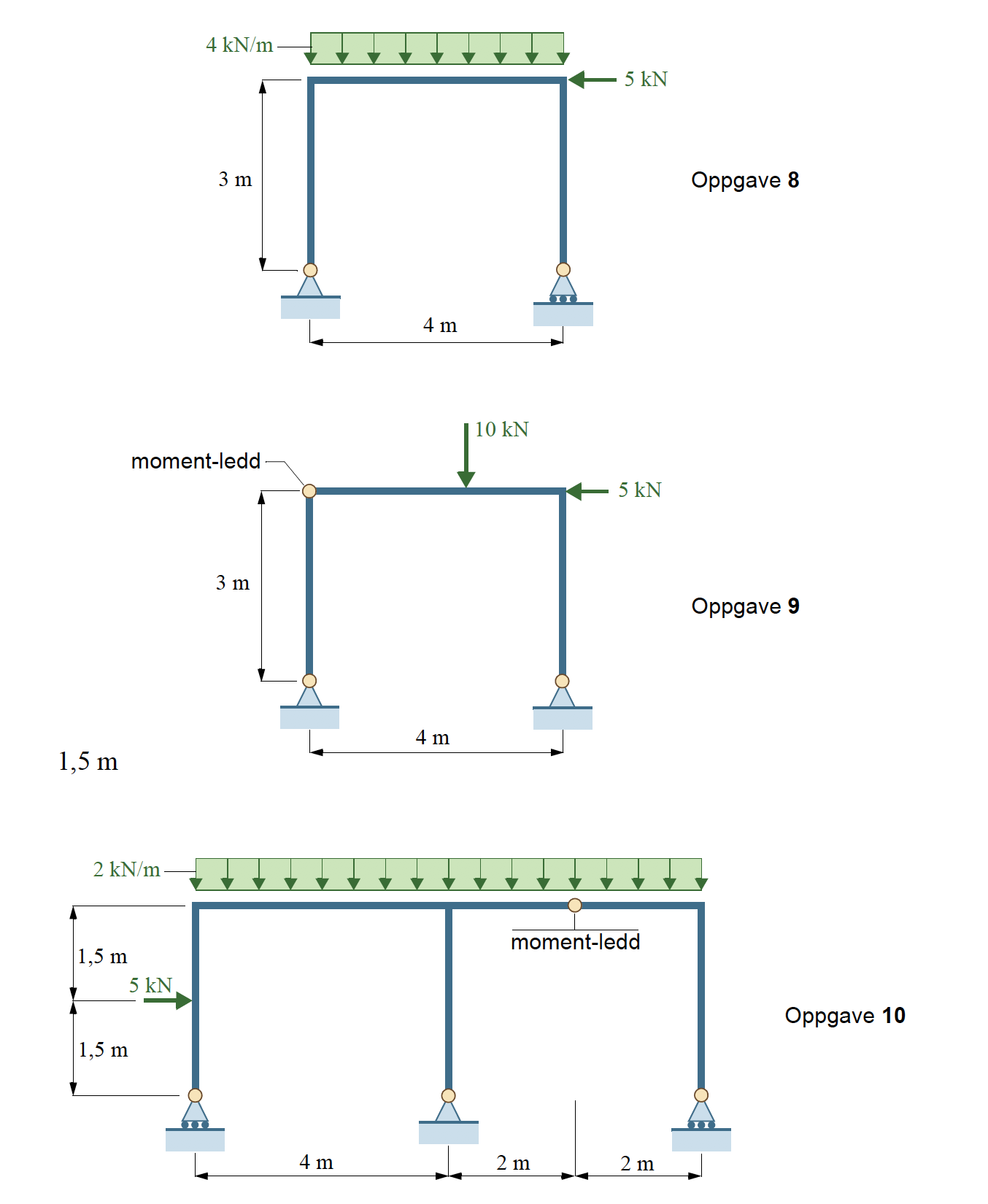
Find the reaction forces, moment and shear-force distribution for the following problems! Document your findings with drawings/sketches.
(Oppgave 1 - 10)
Figure 62: Training excercises: Simple beams. Illustrations from Kolbein Bell.
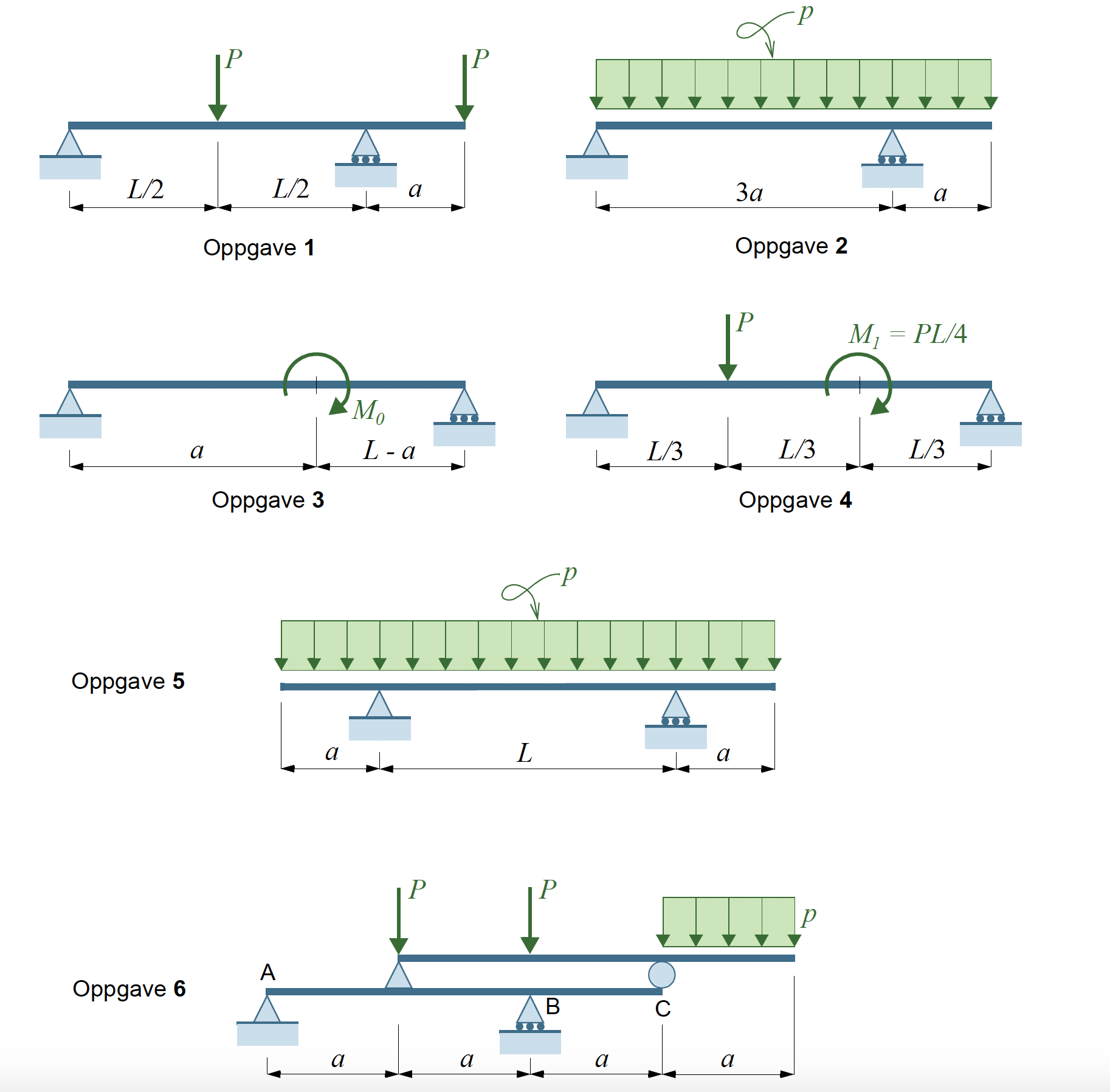
Figure 63: Training excercises: Simple frames. Illustrations from Kolbein Bell.
Lecture 4 - Principle Load Effects in Structures (Part 2)
Vertical and Horizontal Load Bearing in Buildings
A building is a structure with walls, floors and a roof that provides shelter to human activities as e.g. accomondfation, education, production, etc. There is a large varity of buildings and in general some technical installations are included to the buildings.
Figure 64

It is therefore often distiguished between the structural and non-structural part of a building. In this part of the course we deal with the structural part, and allmost all principle structural elements introduced in Lecture 2 are represented in buildings, however, the most relevant are:
- Slabs (as Walls, Floors, Ceilings or Roofs)
- Columns
- Beams
- Rods (mainly for braching)
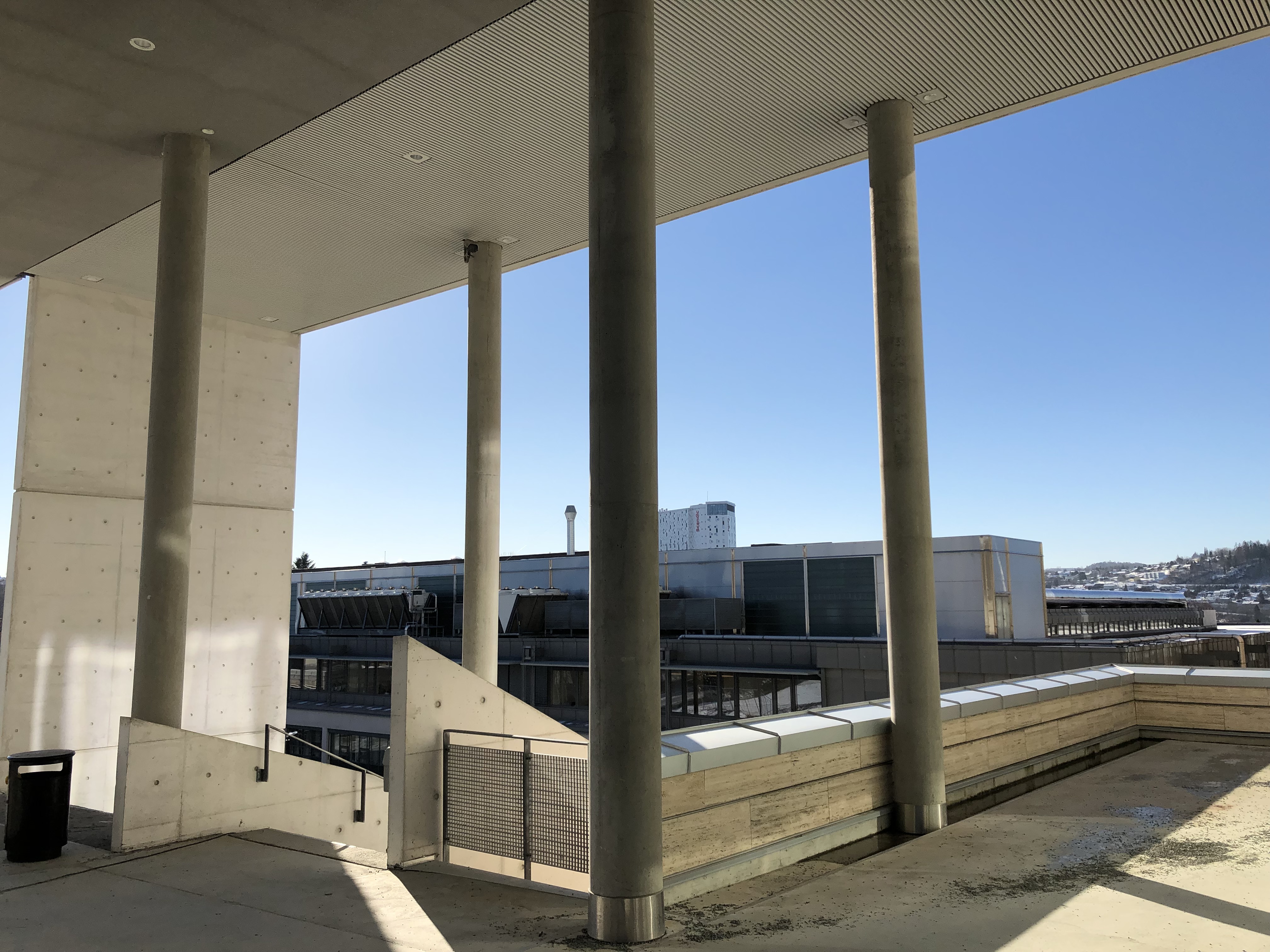
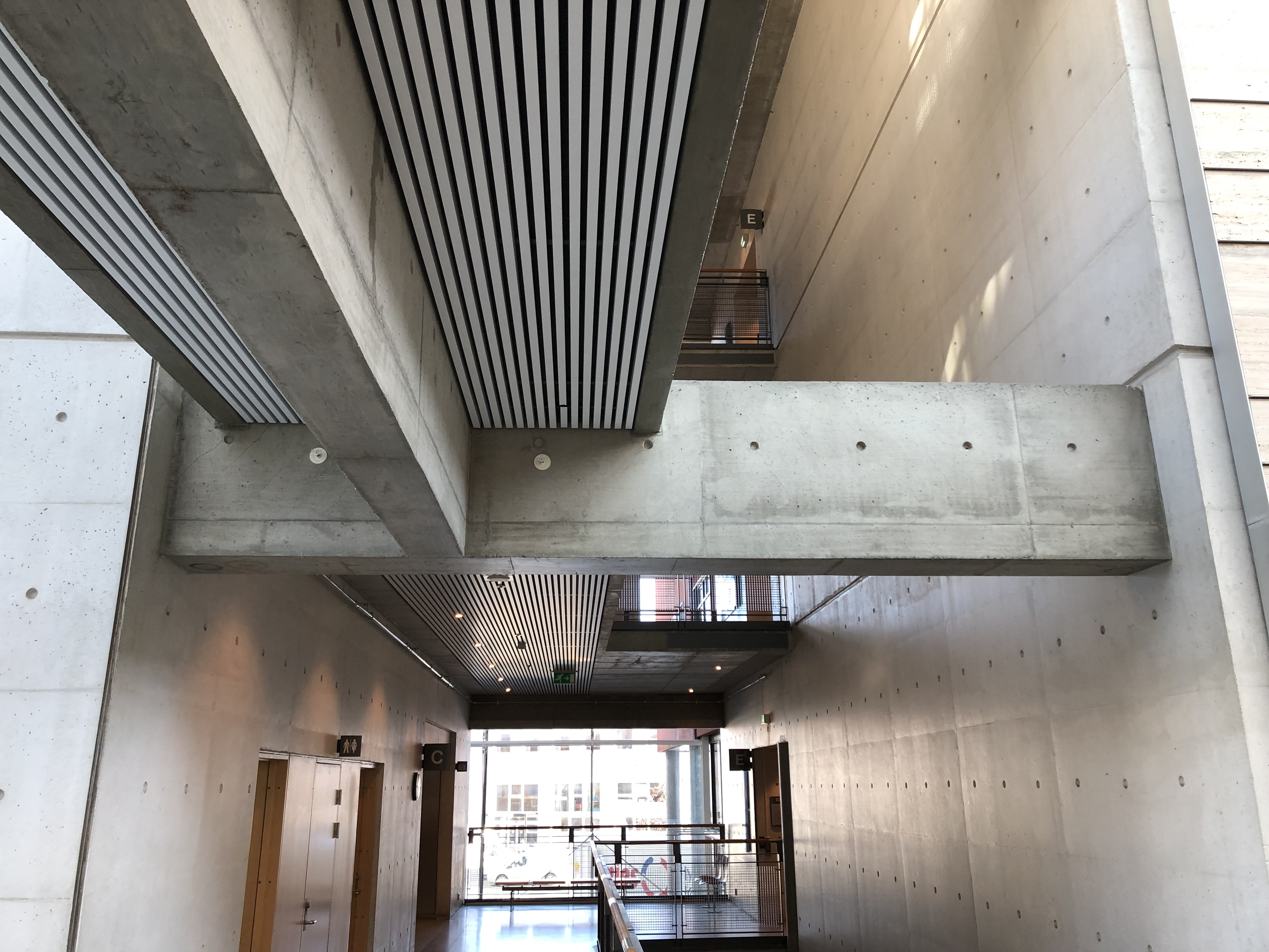
Figure 65: Identify principle structural elements! Where do you see beams, columns, slaps ...? How do they transfer loads into the ground? The image is from the Realfagbygget/NTNU. Go there and look insitu!! Go up the stairs and look for the roof structure as well.

Challenge yourself:
Go to an interesting building (as for instance the Realfagbygget at NTNU). Look out for principle structural elements!! How do they work? how are they loaded? How do they contribute to the load bearing concept of the building?
Make photos, sketches and small descriptions!
Buildings are exposed to Vertical Loads and Horizontal Loads. Horizontal loads are induced e.g. by wind pressure or earthquakes. Vertical loads are dominated by gravity loads, but wind pressure can also induce loads vertically.
Vertical load bearing
Vertical loads in buildings are dominated by gravity loads as:
- Loads from the Self-Weight of structural and non-structural parts of the building
- Loads from any stationary of moving installations or furniture, loads from occupation - these loads are generally referred to as Live-Loads
- Snow-Load
- etc.
Figure 66: Vertical loads from self-weight and live-load are accumulating and can reach very high magnitudes for tall buildings.
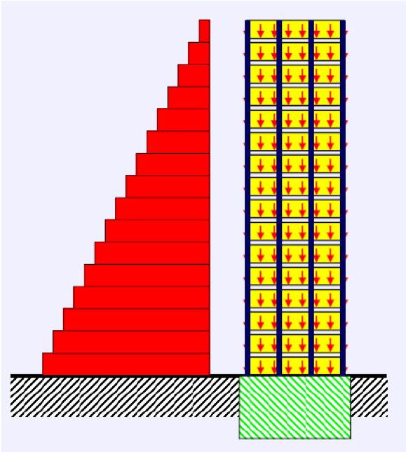
Figure 67: Vertical loads are in general picked up by floor slaps and beams and transfered laterally towards walls and columns and towards the ground foundation.
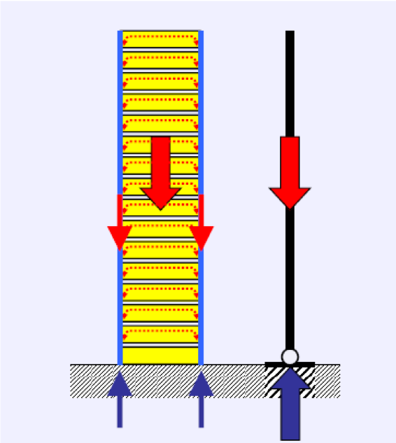
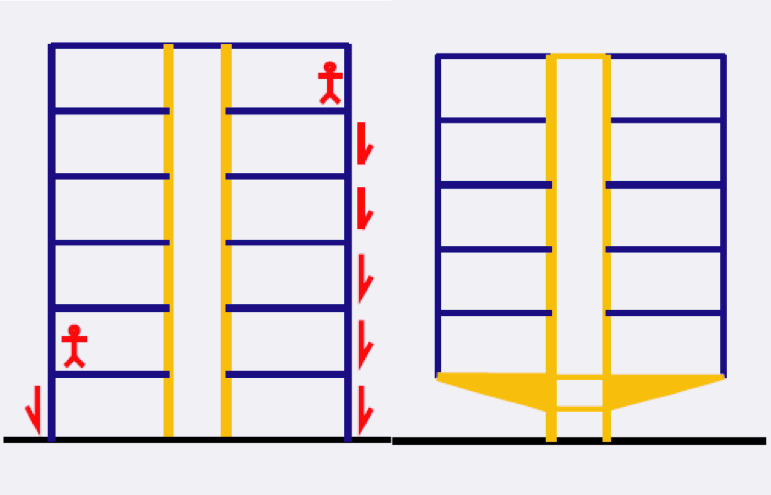
The vertical load transfer should thereby be as simpel as possible. Any opening or disruption of the modular and rectangular shape is causing surplus of loads on individual elements.
Figure 68: Simple is best as seen on the right hand side. Disruptions as openings are unfavorable (middle) or constitute bad structural enginerring solutions. Which elements are most loaded?
The accumalation of vertical loads is crucial for highrise structures, as the large loads demand high loadbearing capacity i.e. large cross-sections for the load transferring elements. The first high rise buildings were build in masonry and here the required dimension of the lowermost walls and columns was a limiting factor. In the lower floors, openings are rare and wall thickness is huge. A good example for this is the Monadnock Building from 1893.
The introduction of stronger materials, i.e. steel and reinforced concrete made it possible to build higher buildings. (See the interesting article about the history of tall buildings).
Large cross-sections restrict the possibilities of openings (e.g. windows and entrance) in a building, which could be disadvantageous - especially for the lower floors of commercial and representative buildings. An interesting solution to that problem is presented in the following image.
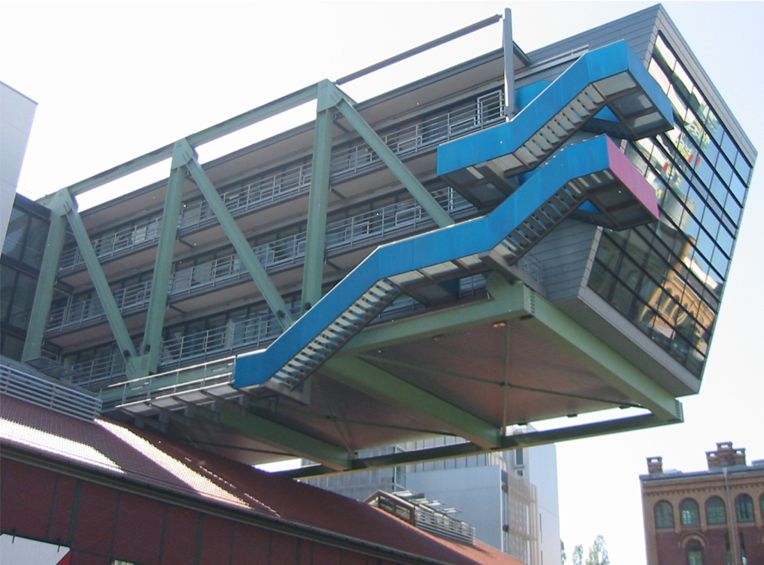
Figure 69: The gravity induced compression forces are transfered by the so called core in the center of the building. The structure is hanging on ropes and tension rods along the facade of the building. The tension rods are not prone to buckling and can be design much more slender compared to corresponding compression elements. Note that this concept provides ample free space at the suterrain level which is beneficial for comercial and representative use.
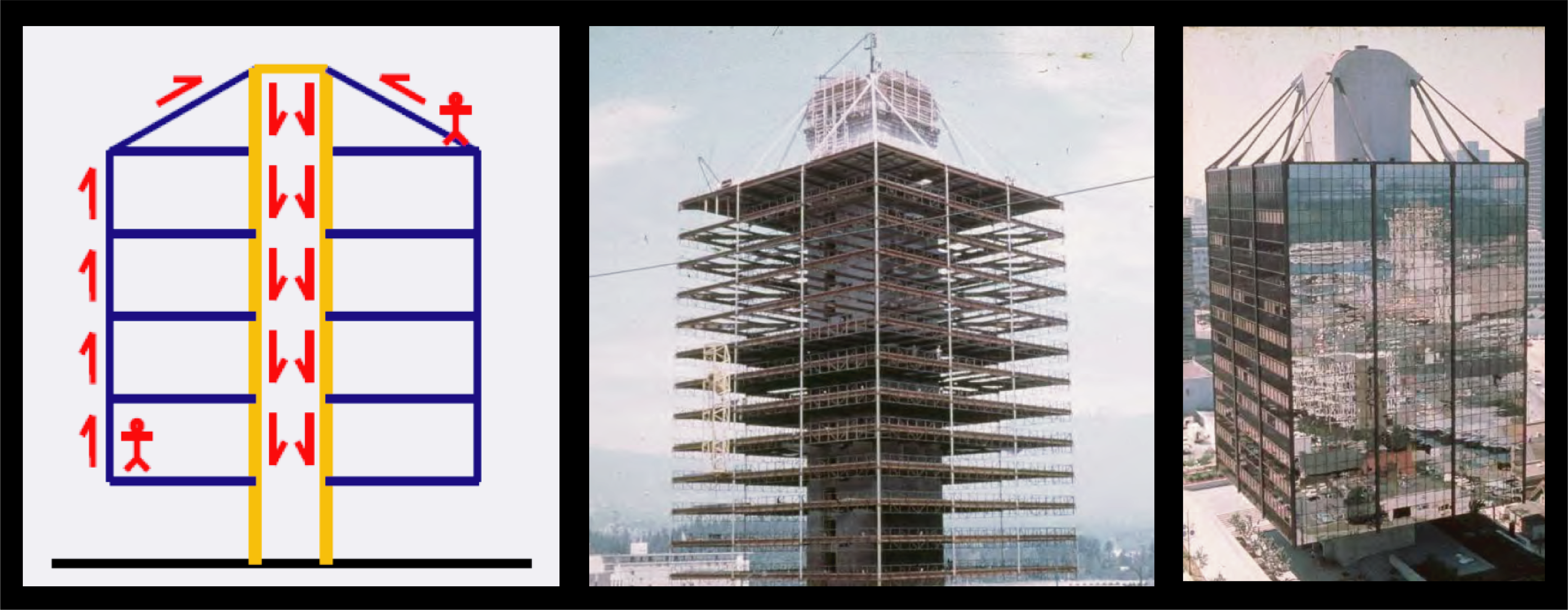
Figure 70: The core-concept is often used in buildings. The core is very often made of reinforced concrete and provides a vertical slot to the building. Staircase and/or elevator are placed well there - also for resons of fire protection.
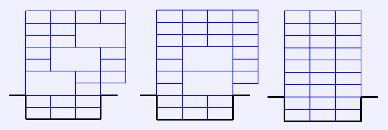
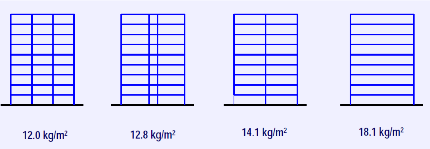
The strategy for vertical load bearing is also influencing the magnitude of vertical loads. In the figure below, four alternative strategies for an 18m wide building are indicated with the corresponding self-weights of the floors. Why are the floor weights becomming larger from the left to the right?
Figure 71: Different strategies for vertical load transfer for a 18m wide building. The floor self-weights are indicated.
Horizontal load bearing
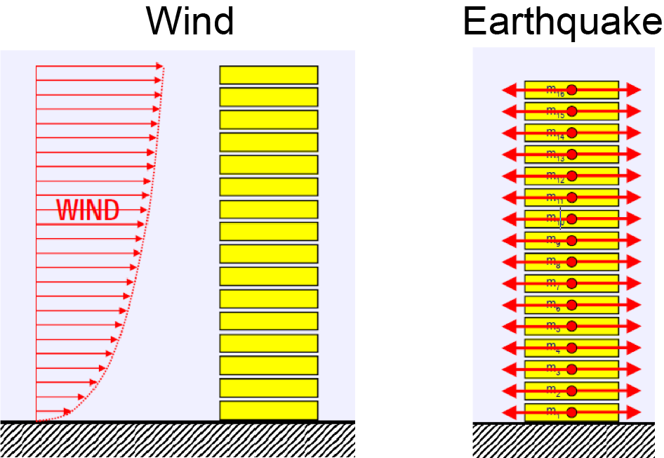
Buildings are also subject to horizontal loading. Typical horizontal loadings to be considered in the design of buildings are wind pressure and earthquakes. Wind pressure yields a distributed loading configuration with magnitude increasing logarithmically with altitude. Earthquakes causes vibration of the foundations of the building resulting in complex dynamic loading of the structure.
Figure 72: Typical horizontal loading in buildings.
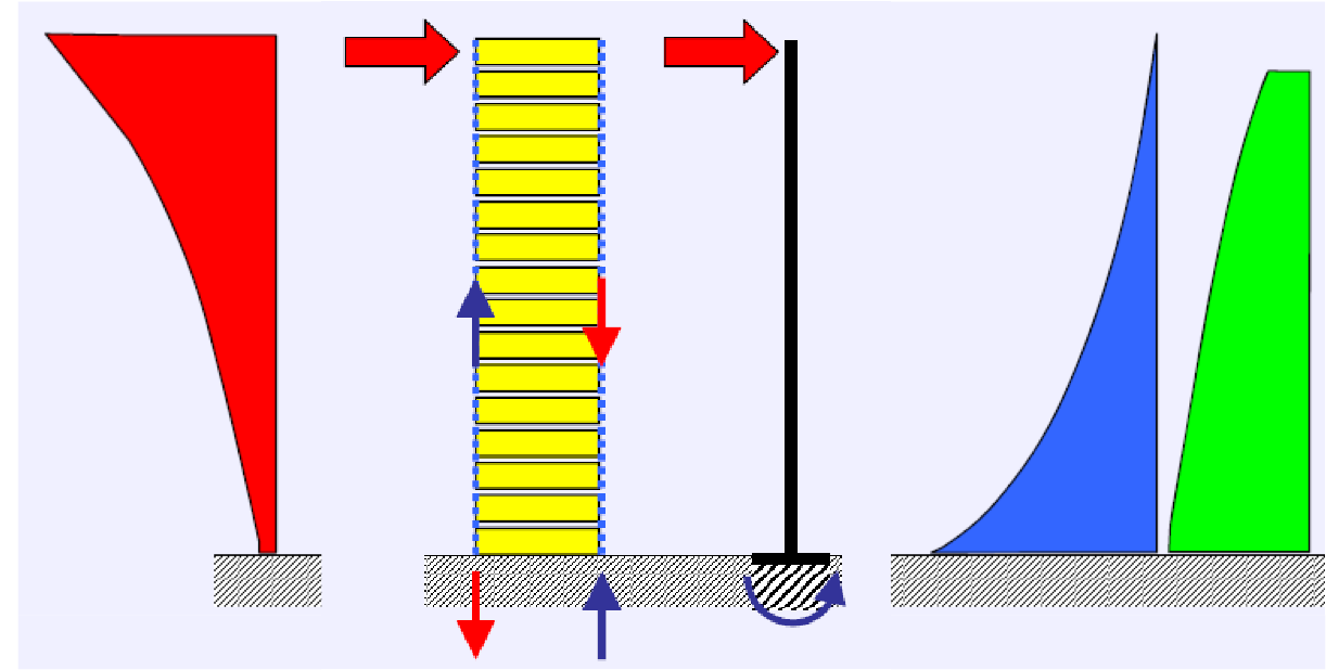
The load effects caused by horizontal loading in buildings can be understood in analogy with loads in a cantilever. The cantilever in the figure below responds to the applied horizontal loading with bending and shear. In a building, this corresponds to tension of the columns of the side where the pressure is applied and the compression of the columns in the opposite side. (Note that the load effects shown are the ones due to horizontal loading only. If they are combined with the load effects induced by vertical loads (by superposition), normaly, no tension in the side columns remains).
Figure 73: Load effects caused by horizontal loading such as wind loading.
Several structural strategies have been developed for efficient horizontal load bearing.
Figure 74: Strategies for horizontal load bearing.
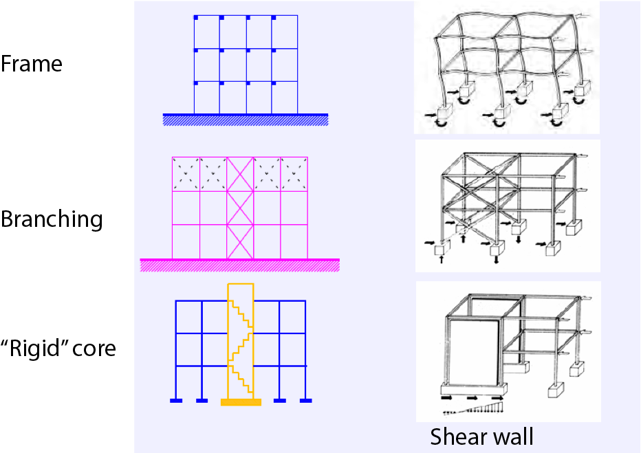
Horizontal loads are transferred from vertical and horizontal shear elements. Rigidity needs to be thought of in three-dimensions in order to provide stability.
Figure 75: Shear walls.
Requirements for stability are summarized as the following rules:
- Minimum three “shear walls”
- Minimum two different orientations of the “shear walls”
- Minimum two intercepts of the “shear wall” directions
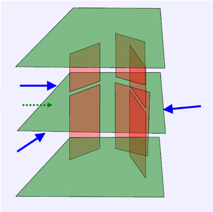
Figure 76: Three-dimensional stability.
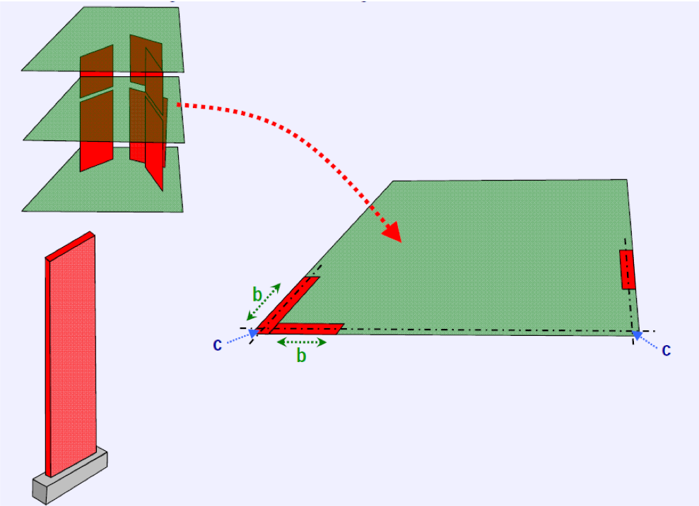
Figure 77: Thre-dimensional stability strategies with shear walls.
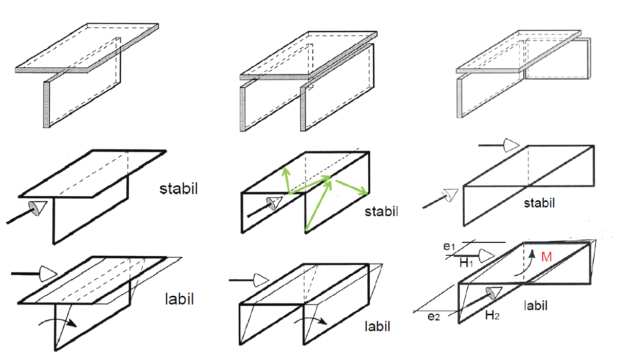
Figure 78: Horizontal load bearing with shear walls.
The rigid core solution works well for both vertical and horizontal loading. A rigid core is typically made of concrete.
Figure 79: Strategies for horizontal load bearing: Rigid core.

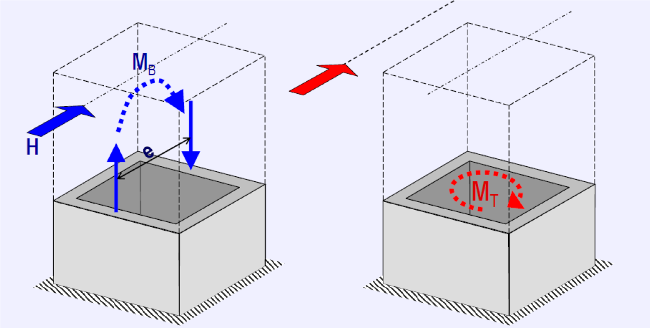
The horizontal loads are transferred to the core, which carries the loads to the ground through bending and/or torsion. Note though that the torsion stiffness is compromised by openings. The vertical elements not part of the core carry usually only normal forces.
Figure 80: Principle of rigid core.
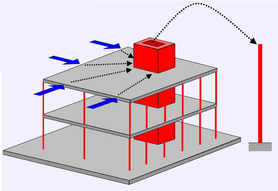
Figure 81: Load effects in the rigid core.
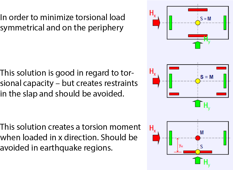
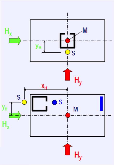
The rigid core works best if placed central. Nevertheless, due to architectural reasons this is not always chosen. If placed in the periphery, large horizontal movements might occur. This can be corrected with an additional shear wall in far distance to the core. (blue)
Figure 82: Arrangement of the core.
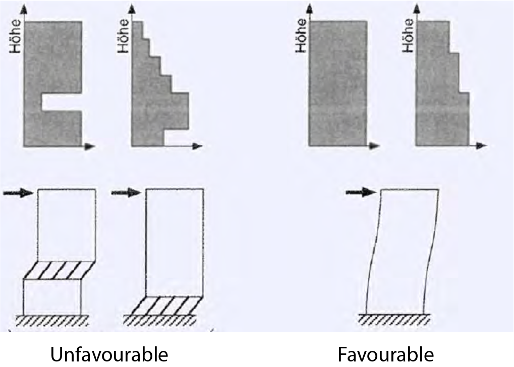
The horizontal stiffness especially of taller buildings should be as uniform as possible. Weak storeys will lead to a inferior structural behaviour.
Figure 83: Distribution of horizontal stiffness in height.
Lecture 5 - Loads on Structures
The learning goal of today is:
- develop a basic understanding about load on structures in general
- understand time variability and return period of extreme events
- quantify snow loads on structures
Reading / Homework:
- Per Kr. Larsen - Konstruksjonsteknikk: Chapters 3.3 + 3.5
- Designers' guide to Eurocode 1
- NS-EN 1990:2002 Basis of Design
- NS-EN 1991-1-3:2003 Snow
Introduction
Loads can generally be categorised as:
- Permanent or variable
- Direct or indirect
- Fixed or free
- Static or dynamic
Loads act on structures as areal forces \( [N/m^2] \) but are also often represented as line forces \( [N/m] \) or point forces \( [N] \).
In building and civil engineering infrastructure, actions are associated to larger uncertainties than the resistance. Loads are uncertain due to:
- Random variations in space and time.
- Modelling: How a physical phenomenon such as wind loading is represented as a simplified mathematical expression introduces large uncertainties.
- Statistical uncertainties.
Loads are very often due to gravity, i.e. due to the weight of matter. Examples for gravity loads are:
- self weight
- snow load
- weight of furniture and installations in buildings
- persons or machinery.
Important loads that do not originate from gravity are wind loads or seismic loads.
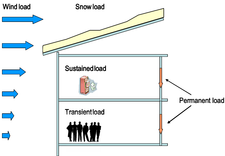
Figure 84: Illustration of different types of loading on a building.
Despite the large uncertainties and variabilities that are associated to the quantification of loads, in structural design codes as the Eurocode loads are represented by single values, the so-called characteristic values. The definition of characteristic values is specified in the code – in the Eurocodes loads are represented as follows:
- Permanent loads are represented with mean values.
- Time variable loads with the extreme value with 50 years expected return period (98%-fractile of the yearly extreme value distribution).
Representation of time variable loads
A time variable load is a load that changes its magnitude discretely or continuously over time. A realisation at a certain point in time can in general not be predicted with certainty, however, its variability can be expressed and this is in general done by a random process. Random processess can be characterised by mean value, standard deviation and autocorrelation. For structural engineering purposes it often sufficient to represent random process by their corresponding extreme value distributions. The extreme values are thereby defined as the distribution of maximuma eller minima observed (or expected) in periods of specified equal duration. E.g. if the specified period is one year, then a observed process of 50 years would feature 50 observations of yearly maxima. Such data might be used for finding a distribution that represents the distribution of future yearly extreme values under the following critical assumptions:
- the reference period is chosen long enough such that the single observations of extremes can be considered as independent. (this would obviously not be the case if a period shorter than 1 year is chosen for climatic actions)
- The random process is ergodic - this means, broadly spoken, that the statistical properties of the properties remain the same over time.
The first assumption is valid if the reference period is carefully chosen. For climatic actions as snow and wind it is in general assumed that one year is long enough. However, for live loads that include furniture in buildings 1 year is apparently not long enough as the arrangement of furniture renews with a smaller rate than one year. Thus for live loads longer reference periods, as e.g. 5 years are generally used.
The second assumption is more crucial due to obvious reasons:
Challenge yourself:
One main assumption that extreme realisations of a load can be represented by single random variables is that the random process is ergodic. Why is this an assumption that is hardly valid (in a strict sense) for any time variable load process? Discuss them with your fellow students!
As previously mentioned, the characteristic value of a variable load is defined as the 98%-fractile of the yearly extreme distribution. The values are dependent on the geographical region for environmental actions as snow or wind, and dependent on the use of the building for live loads in buildings. Values are given in tables in the Eurocodes for different geographical regions and different uses of buildings. The values are identified based on observations and corresponding extreme value statistics.
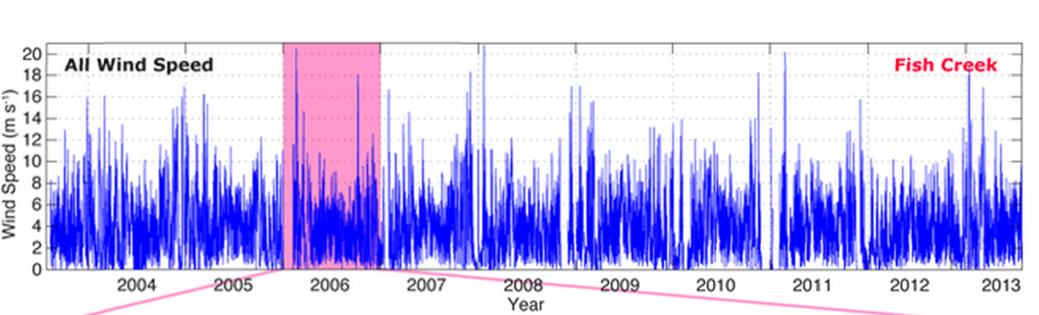
In Figure 85 the record of wind speed data of "Fish Creek" is displayed. A yearly pattern with larger realisations in the winter season can be identified. Each yearly maximum can also be seen - these values would be the basis for the establishment of a yearly extreme value distribution.
Figure 85: Time series of the wind wind speed over a decade.
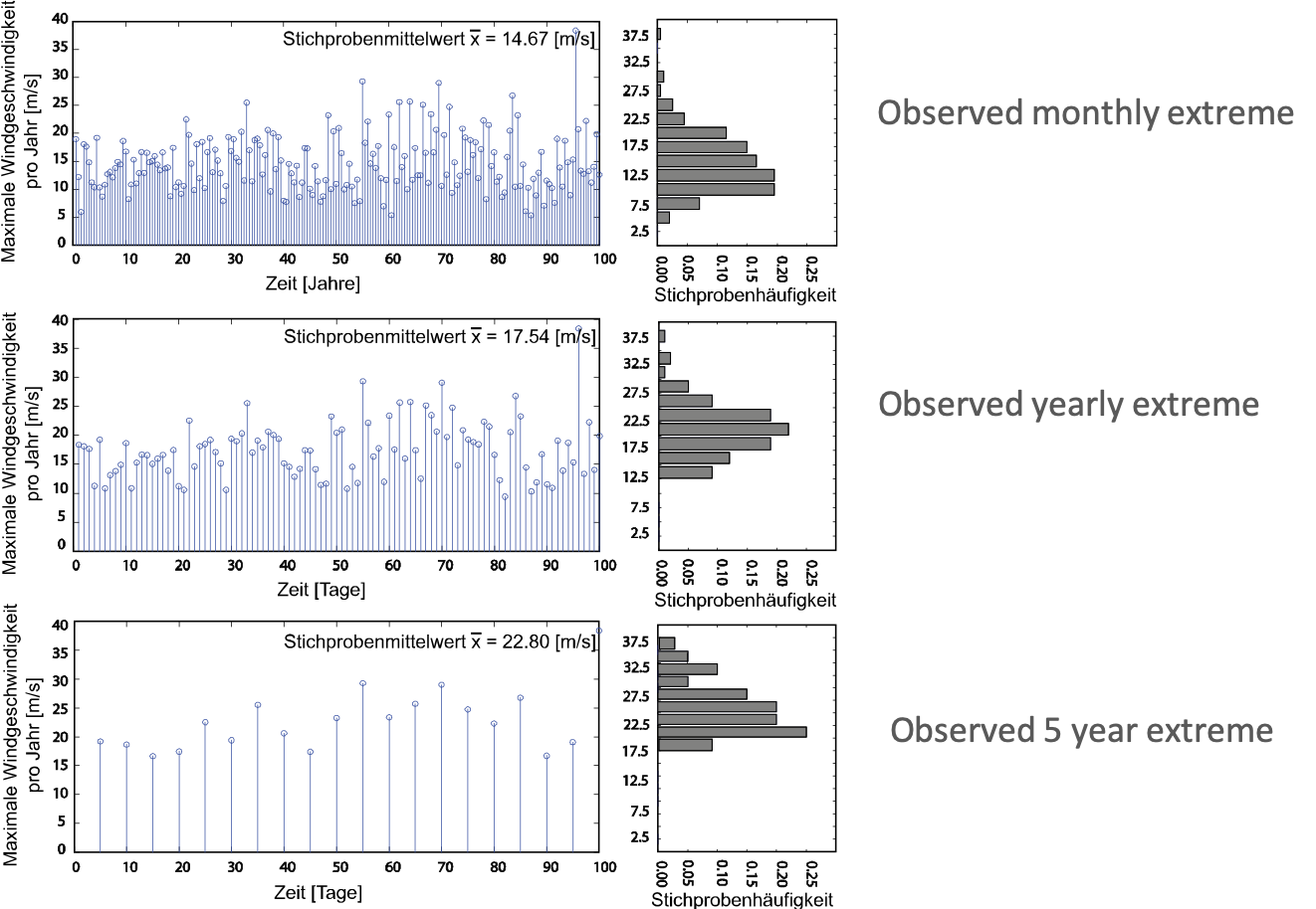
The extreme value distribution is dependent on the specified reference period, in longer periods it is more likely to observe larger values. This phenomenon can be observed in Figure 86.
Figure 86: Extreme value distributions for different reference periods given 100 years data.
Time dependency
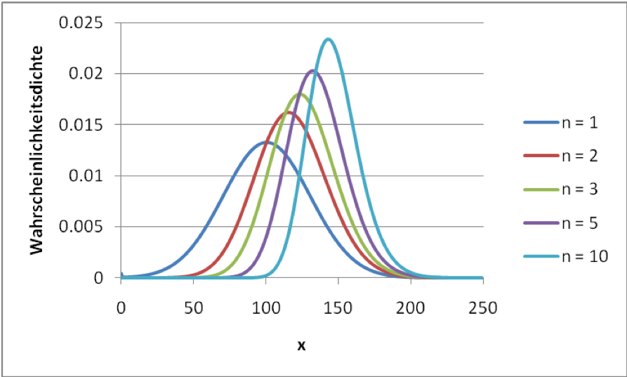
Assuming the extreme values within a period \( T \) of an ergodic random process \( X(t) \) are independent and follow the probability distribution \( F_{X,T}^{max}(x) \), the extreme values of the same process within the period \( n\cdot T \) follow a distribution:
$$ \begin{equation}\label{eq:Extremedependency} F_{X,nT}^{max}(x) = (F_{X,T}^{max}(x))^n \end{equation} $$The effect can nicely be seen in Figure 87.
Figure 87: Scaling of the extreme value distribution for different reference periods \( n\cdot T \).
Characteristic value
The characteristic value for time variable loads \( x_k \) is defined as the \( 98\% \) fractile of the yearly extreme value distribution meaning that this value has a yearly non-exceedence probability of \( 0.98 \), or a yearly exceedence probability of \( 0.02 \) correspondingly, i.e.
$$ \begin{equation}\label{eq:98fractile} F_{X,T=1}^{max}(x_k) = \Pr(X\leq x_k) = 1- \Pr(X > x_k) = 0.98 \end{equation} $$Thus, the probability to observe a value larger than \( x_k \) is \( 0.02 \) per year and the probability to observe a maximum value per year less than \( x_k \) is \( 0.98 \). The probability to observe a two year maximum value less than \( x_k \) is \( 0.98 \cdot 0.98 = 0.9604 \) (the two year exceedence probability for \( x_k \) is then \( 1-0.9604=0.0396 \)). Extending the reference period to \( n \) years the non-exceedence probability is \( 0.98^n \) and the exceedence probability \( 1-0.98^n \) correspondingly.
Return period
The return period is a frequency measure that is often used to express the likelihood of an event. As the name implies, the return period specifies the expected waiting time between (the return) of an event. An event may be defined as the exceedence of the characteristic value as described above. Or vice versa, how frequent would we observe an event with a yearly probability of \( 1-F_{X,T=1}^{max}(x_k)=0.02 \)? The corresponding return period is:
$$ \begin{equation}\label{eq:RefPeriod} T_{R} = \dfrac{1}{1-F_{X,T=1}^{max}(x_k)}=\dfrac{1}{0.02}=50 \end{equation} $$Snow load
Figure 88: Snow load.

Introduction
In central and northern europe snowload is often the dominant load on building roofs. Pursuing a realistic modelling of the snow loading is a complicated task. Snow fall is a complicated phenomenon that is influenced by many parameters. In addition, the snow load pattern on a roof is redistributed due to factors such as the roof inclination or the wind. Fortunately, it is not necessary nor fruitful to deal with a lot of detail for the design of building and other constructions. We are rather more interested in identifying the extreme load effects. Structural standards as the Eurocode prescribe (in the form of tables in the National Annexes) the characteristic values of the snow load on the ground at different geographical locations. These values are then altered by factors that account for some of the most relevant influencing factors to compute the characteristic snow load on buildings.
Snow load on the ground
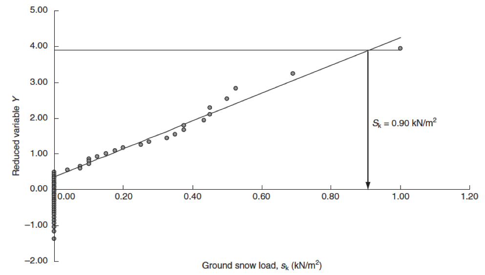
The estimation of the snow load on a structure takes the snow load on the ground as basis. Symbol: \( s_{k,0} \). It is expressed in \( \text{kN/m}^2 \). The snow load on the ground is based on collected data. The typical observation period is 100 years. \( s_{k,0} \) is given in the National Annex (NA) for different geographical regions. The characteristic value represents the 98% fractile value of the yearly extreme distribution (50 years return period). The 98% fractile value is often computed assuming a Gumbel Type I least squares fit of the observed data. This can be seen in Figure 89.Figure 89: Probability paper (Gumbel Type I) for the weather station at Arezzo, Italy. Source: Designers' guide to Eurocode 1.
Altitude correction
Figure 90

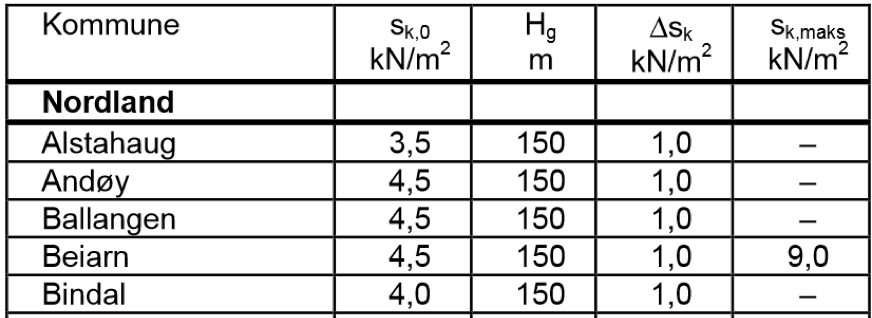
The snow precipitation typically increases with the altitude. In the Norwegian national annex in the Eurocode, the following linear scaling expression is provided to estimate the snow load at a certain altitude:
$$ \begin{equation}\label{eq:s_k} s_k = \min\{s_{k,0}+n\Delta s_k;s_{k,maks}\} \end{equation} $$Note that \( n \) is always rounded up to the next larger integer. The scaling is applied for \( H>H_g \). \( H_g \) is the reference height up to which \( s_{k,0} \) can be used as the characteristic value of snow on the ground at the building location. \( s_k \) is sometimes topped by a maximum value \( s_{k,maks} \).
$$ \begin{equation}\label{eq:n} n = \dfrac{H-H_g}{100} \end{equation} $$All these values are tabled in the Eurocodes for different geographical regions - in Norway per Kommune.
Figure 91
Snow load on buildings
Snow can be deposited on a roof in many different patterns. The pattern depends on the wind exposure but also on:
- Shape of the roof
- Thermal properties
- Surface roughness
- Surrounding terrain and buildings
The Eurocode EN1991 provides the following simplified formula to take these factors into account:
$$ \begin{equation}\label{eq:s} s = \mu_i C_e C_t s_k \end{equation} $$Where:
- \( s_k \): characteristic snow load on the ground.
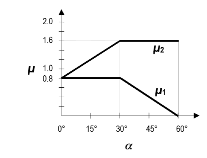
- \( \mu_i \): snow shape coefficient. It depends on the roof inclination, see Figure 94. This factor is elaborated further below.
- \( C_e \): exposure coefficient. This coefficient depends on the surrounding topography and it accounts for the displaced snow due to wind. The topography is divided into three categories: (a) Windswept; (b) Normal; (c) Sheltered. It is required to consider the future development of the area where the construction is going to take place.
- \( C_t \): thermal coefficient. It is often set to 1 as a conservative assumption. It accounts for the snow that may be melted due to heat transferred from the building.
Snow distributes differently depending on the shape of the roof. It is general distinguished between undrifted and drifted states. Undrifted describes the situation of snow uniformly distributed on the roof. Thus, the snow pattern is only affected due to the gravitational redistribution due to the shape of the roof in this case. Drifted describes the situation in which snow is transported from one location to another due to e.g. wind.
Figure 92: Snow can be drifted by the wind and this creates asymmetrical loading. Some structures are quite sensitive to asymmetric loading.
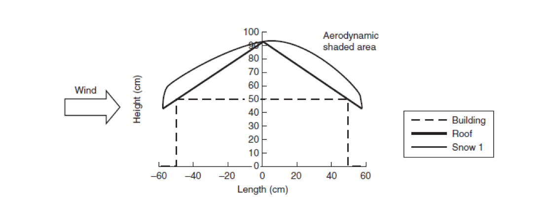
Figure 93

Figure 94: \( \mu_i \) coefficient as a function of the roof inclination \( \alpha \).
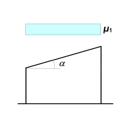
Pitched roofs
For single pitched roofs there is no distinction between drifted and undrifted. The pattern is shown in Figure 95.
Figure 95: Snow load pattern for single pitched roofs.
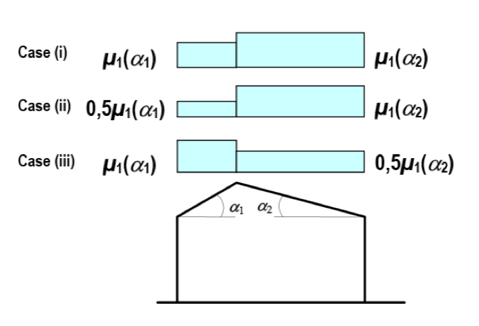
For double pitched roofs there is a distinction between drifted and undrifted. The pattern is shown in Figure 96.
Figure 96: Snow load pattern for double pitched roofs.
Multi-span roofs
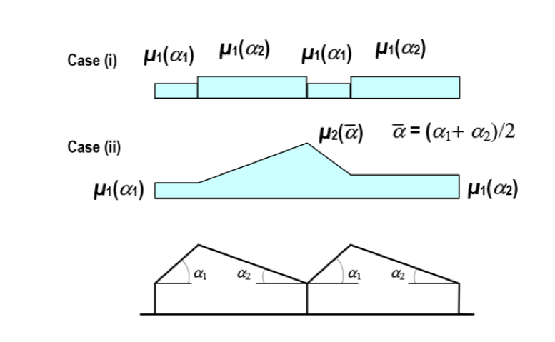
Two situations are considered for multi-span roofs, see Figure 97. Note that for the case of V-shaped roof, the coefficient \( \mu_2(\bar{\alpha}) \) applies, with \( \bar{\alpha} \) being the average angle of the two neighbouring inclined roofs.
Figure 97: Snow load pattern for multi-span roofs.
Roof abutting and close to taller construction works (drifted case)
Figure 98

Snow might drift from a neighbouring higher roof. Snow accumulation in the lower roof is considered to be the result of snow sliding and wind:
- sliding of snow from the upper roof, \( \mu_s(\alpha) \) (see Clause 5.3.6 in EN1991-1-3)
- accumulation induced due to wind, \( \mu_w \):
Figure 99: Snow load pattern for roof abutting.
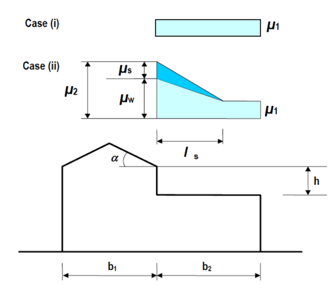
Where \( \gamma \) is the weight density of the snow. It can be assumed to be \( 2\text{kN/m}^3 \). The length \( l_s \) can be estimated as \( l_s = 2h \). Limitations are covered in the national annex.
Lecture 6 - Wind loads
Wind loads
Introduction
Wind is generally understood as the bulk movement of air in the atmosphere. Winds are the result of
- large atmosphric circulation due to diffrent heating at the equator and in the polar regions,
- more local phenomena due to corresponding local temperature gradients particulary observed at the interface of big land and water mass or in mountain regions, and,
- the physical shape of the surface on different scales, oceans, lakes, planes, mountain ranges, valleys, down to the terrain roughness and buildings.
Winds are often refferred to according to their strength (speed) and direction from which the wind is blowing. The wind speed at a point on the earth surface is a very time variant phenomena. Short bursts of a view seconds are termed gusts, medium long periods (around one minute) of high wind speed are refferred to as squals. Medium - long duration wind events are called, dependent on their average strength, breeze, gale, storm. Very strong storms of catastrophic intensity are generally refferred to as cyclones, but also called hurricanes or typhoons.
Looking at the weather development over time (just play the video). Clear patterns are visible together with a strong random/chaotic component.
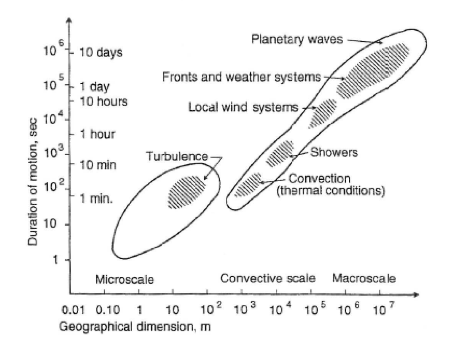
Figure 100: Wind speed is highly variable phenomena over time. The time variability is following a pattern related to the different origins of the variability. Here, the atmospheric processes, single weather systems, single weather events, local turbulences.
An interesting clip that illustrates the effect of the terrain on local wind phenomena.
Definition and characteisation of wind as a structural load
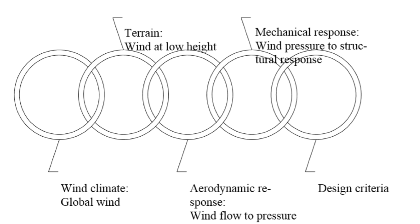
In order to characterize the relevant wind load effect on structures the wind speed is only one of many relevant features to consider. The shape and the roughness of the local terrain is important to consider as it might more or less disturb the laminar flow of air, the shape of the structure, that can be seen as a obstacle in the wind stream is determining the pressure the wind induces to the structure. The pressure pattern on the surface of the structure has finally to be transfered to a structural respons that is either considered static or dynamic. A schematisation of wind load modelling is illustrated in Figure 101
Figure 101: The wind modelling chain.
Wind speed
In the Eurocodes (EN1991-1-4) different geographical locations are associated with a corresponding reference wind speed, \( v_{b,0} \) that is defined as:
Reference wind speed: Charcteristic 10 minute average windspeed measured 10 meters over the ground in flat terrain with low vegitation and obstacles in a distance lager than 20 times their height. The reference wind speed corresponds to the 98% fractile of the yearly extreme value distribution.
The reference wind speeds are tabulated in the national annex of EN1991-1-4, e.g. some values for Norway as follows:
Figure 102
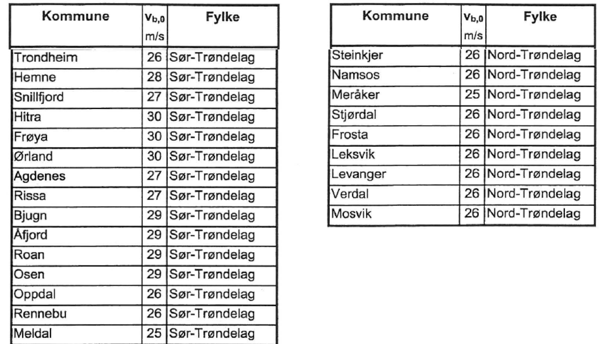
Basic windspeed: The basic wind speed \( v_b \) is computed based on the reference wind speed \( v_{b,0} \) as
$$ \begin{equation}\label{eq:basespeed} v_{b}=c_{dir}c_{season}c_{prob}v_{b,0} \end{equation} $$\( c_{dir} \) is a possible correction factor for the wind direction, \( c_{season} \) a correction factor for different seasons, and \( c_{prob} \) is a correction factor if a different design service life than 50 years is used in the basis of design of the corresponding structure at hand. The default of all correction factors is 1.0 and this value should be used unless very good argument can be made to change the default value.
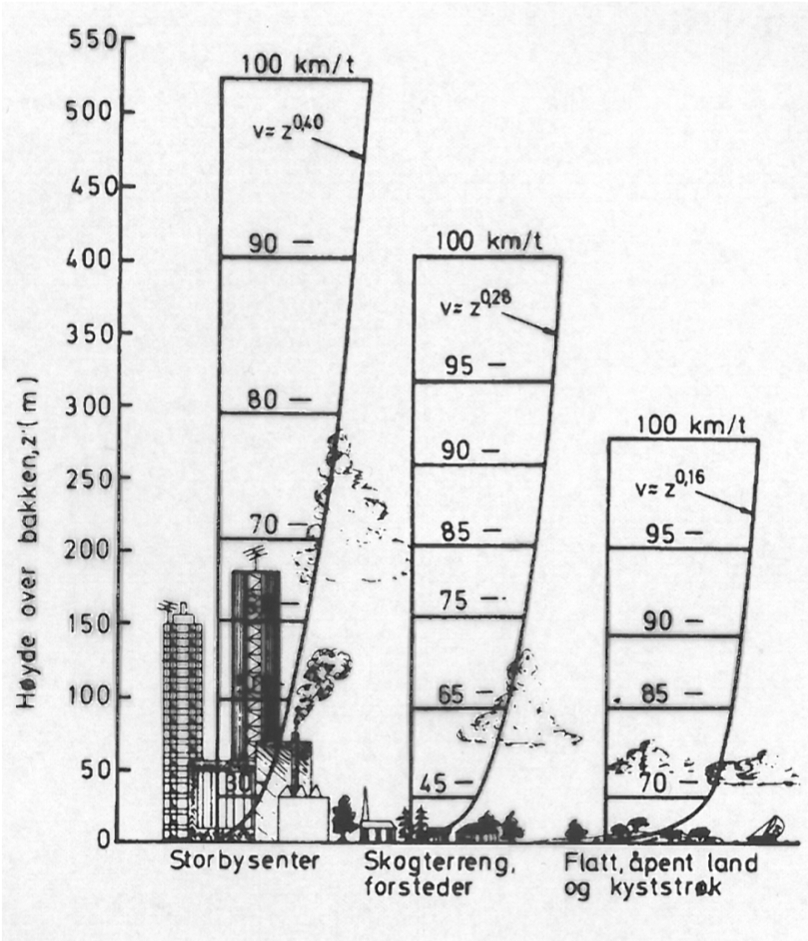
The windspeed is increasing with the height over the terrain due to friction. The distribution over the height of the building depends on the surrounding terrain characteristics.
Figure 103: Windspeed, height and terraincharacteristics.
Wind pressure.
Wind is acting on surfaces of obstacles as a pressure. This pressure is alllways directed in perpendicular direction to the surface! This pressure \( p_w \) is proportional to the square of the wind speed \( v_w^2 \) and for a plane surface it is computed as
$$ \begin{equation}\label{eq:pressure} p_w=\frac{1}{2} \rho \cdot v_w^2 \end{equation} $$, where \( \rho \) is the air density.
This is the wind velocity pressure. The relevant wind speed for the pressure estimation is related to the basis wind speed. However, local terrain shape and roughness and turbulences have to be considered in order to obtain a reasonable estimate for a structure at hand. In the Eurocodes, two alternative options are suggested for this: a detailed alternative where many possible specific aspects can be considered in the estimation, or a simplified alternative where the peak velocity pressure is estimated with a graph that is valid for a specific basis vind speed. In this course, we will stick to the simplified alternative that is introduced in the following.
Simplified estimation of the peak velocity pressure:
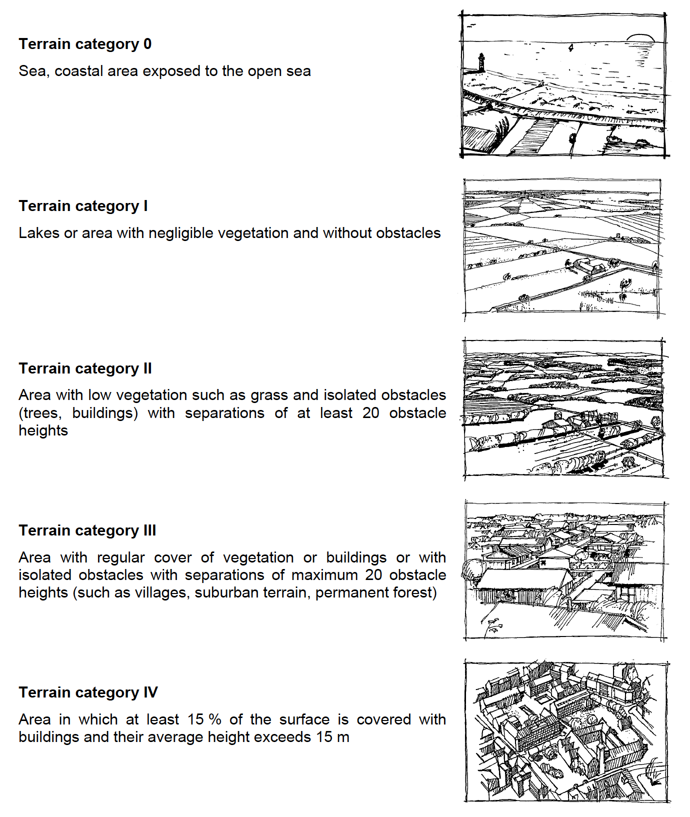
The estimation of the peak velocity pressure takes basis in the basis vind speed \( v_b \) and a graph that describes the interrelation between the terrain characteristics, the height \( z \) of a building and the corresponding peak velocity pressure \( p_{p0}(z) \). The terrain characteristics are classified in 5 different categories, see Figure 105. .
Figure 104: Windspeed, height and terraincharacteristics.
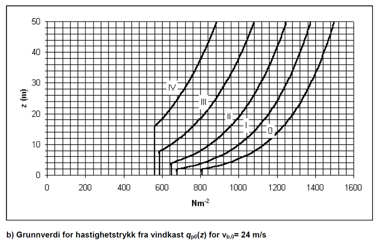
Figure 105: Windspeed, height and terraincharacteristics.
The peak velocity pressure corresponds to the pressure on a standard surface that spans in perpendicular direction to the wind direction. The pressure distribution on the building is estimated based on the peak velocity pressure and a pressure coefficient that is dependent on the shape of the building/structure and its orientation to the wind.
Wind pressure on structure:
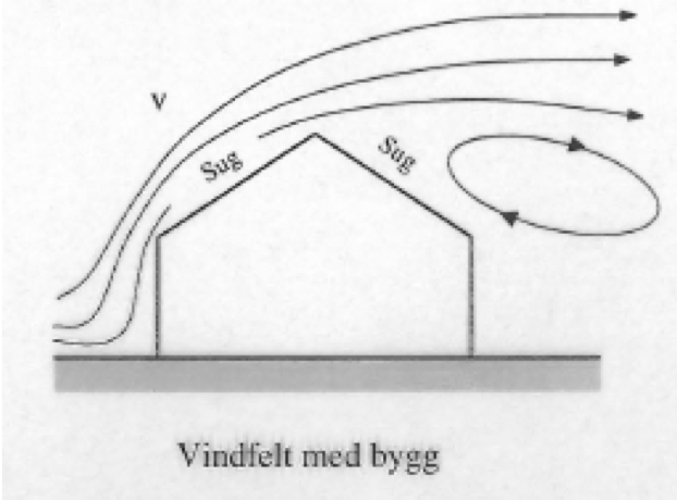
A structure and building is an obstacle to the wind, i.e. to the undisturbed wind field. In Figure 106 the wind direction and velocity is represented by arrows ands their distance, which is proportional to the distance between the arrows. On the left hand side the wind field is undisturbed and the wind goes straight with constant velocity. On the right hand side, The wind flow is disrupted by the structure - the wind has to go around. It can be seen that the distance between the arrows is varying - decreasing distance means acceleration and vice versa. The direction change of airflow together with the different wind speeds creates either positive or negative pressure on the surface of the building.
Figure 106: Illustration of windspeed variation around buildings.
In order to get an idea about basic aerodynamic effects on buildings it is recommended to watch this interesting movie.
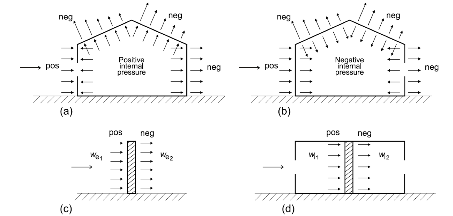
Openings in buildings create particular pressure patterns that have to be considered.
Figure 107: Pressure distribution for structures with openings (From EN1991-1-4).
Dependent on size and shape of the building/obstacle and dependent to the orientation to the wind different pressures might occur.
Wind pressure estimation according to EN1991-1-4.
The estimation of wind pressures on building surfaces is a complex task that in general requires advanced fluid dynamical analysis. As seen it depends on the building shape and wind direction. Moreover, it is dependent on the properties of the wind field the structure is embedded in. Thus, it depends on surrounding buildings and on the terrain.
In EN1991-1-4 simplified and generalised rules for the estimation of the wind pressure are given. The facilitate straight forward assessment of wind loads buildings of simple shape.
Wind pressures on buildings according to EN1991-1-4 are estimated based on the peak velocity pressure \( p_{p0}(z) \) and a pressure coefficient \( c_{pe} \). \( c_{pe} \) is dependent on the building shape and orientation in the wind. Pressure coefficient \( c_{pe} \) is estimated based on EN1991-1-4 section 7.2. This section is very comprehensive and its content is not repeated here.
Lecture 7 - Safety and Structural Reliability
The learning goal of today is:
- develop a basic understanding about safety and structural reliability
- be able to compute the failure probability of a simple structure (with simplifying assumptions)
- be able to connect reliability and the safety factor concept form structural design codes.
Reading / Homework:
- This lecture notes
- Recapture Per Kr. Larsen - Konstruksjonsteknikk: Chapters 1 + 2
- Jörg Schneider - Safety and Reliability of Structures: Chap. 4.31 – 4.33
- Designers' guide to Eurocode 0
Safety - a requirement for structures
The built environment, i.e. infrastructural elements, industrial buildings and facilities as well as residential buildings, constitutes the basis for our economy and the continuous development of our society. In this respect structures play an important role, since the primary purpose of structures is to provide the functionality of the built environment. That structures are safe is an important premise for the success of our society, and structural safety is clearly a basic requirement of the society.
Correspondingly, structural safety is a requirement that is defined in legislation on several hierarchical levels – structures have to be safe by law.
Several formal definitions of safety exist and accordingly, safety is used as absolute or relative characteristic in our regular language use. (“It is safe to use air traffic” is an absolute statement; “Air traffic is safer as car traffic” is a relative statement). In the context of structural engineering the following definition can be found in ISO 2394:2015 :
2: ISO 2394:2015: General principles on reliability for structures.
Structural safety: “ability of a structure or structural member to avoid exceedance of ultimate limit states , (…), with a specified level of reliability, during a specified period of time.”}
3: The exceedance of an ultimate limit states corresponds e.g. to structural failure.
Structural reliability per time unit is defined as the complement of probability of structural failure per time unit; i.e. structural safety is an absolute description for situations where the probability of failure per time unit is sufficiently low.
Attaining structural safety:
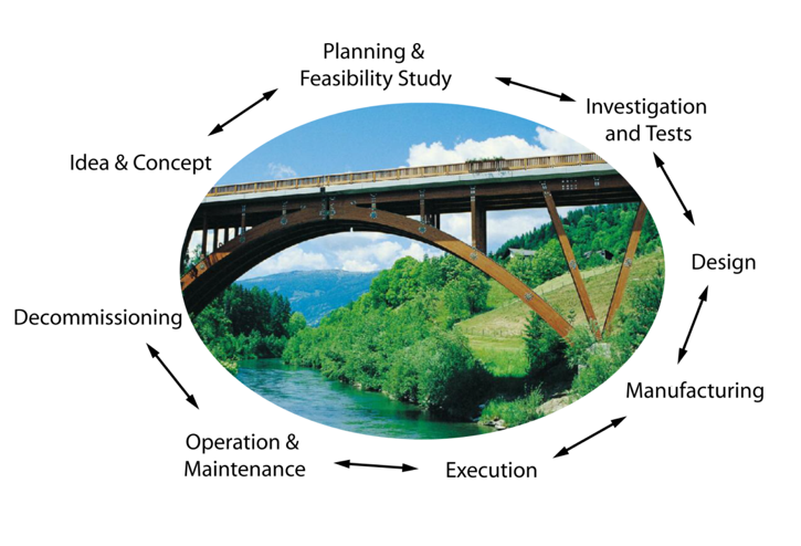
Structural engineers are responsible that structures are safe. Structural engineers therefore make proper decisions during the entire life-cycle of the structure. The typical phases of the life-cycle of civil engineering infrastructure are illustrated in Figure 108.
Figure 108: The life-cycle of engineering structures.
For decision making, structural engineers take into account information e.g. about:
- Traffic volume
- Loads
- Resistances (material, soil, ...)
- Degradation processes
- Service life
- Manufacturing costs
- Execution costs
- Decommissioning costs
As a matter of fact, the information that has to be integrated is associated with uncertainties . Thus, the uncertainties have to be taken into account in the decisions that are made in the life-cycle of the structure.
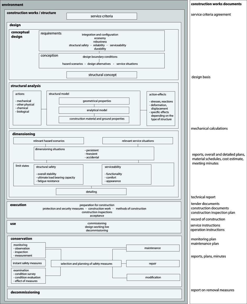
The activities and the decision making of structural engineers are very well illustrated in the Swiss structural standard SIA 260 with the graph presented in figure 109. Here, a structure is defined by its service criteria and the environment it is embedded into. The structure then has the following phases during its life cycle:
- design
- execution
- use
- conservation
- decommissioning
In this course we will focus on the design phase of the structure. In figure 109 the design phase is further subdivided into "conceptual design", "structural analysis" and "dimensioning".
In conceptual design a structural concept is developed that is best to meet the requirements to the structure, i.e. in regard to the intended societal activity that should be supported by the structure these are requirements in regard to
- space and shelter created by the structure,
- requirements on limitation of vibrations and deflections (serviceability),
- requirement on the durability of the structure and the intended service-life.
- safety, i.e. preventing damage, loss of functionality, damage to the environment and to personnel,
- cost efficiency.
In the conceptional design phase, major decision are made in regard to principle structural layouts and material use. Build-ability is always a very important aspect here. Structural analysis is intended to create a link between the external loads on the structure and the corresponding structural response in terms of stresses, deformations and deterioration. Mechanical models (analytical and numerical) are utilized and structural analysis is generally performed at a rather high level of modelling detail.
For structural dimensioning the structural dimensions are chosen such that the structure complies with some specified limit states regarding safety and serviceability. The compliance is demonstrated for several load scenarios ("design situations").
In general it can be observed that the effort and level of detail is not consistently distributed among the different steps of structural design: Whereas a lot of attention is attributed to structural analysis, rather rudimentary criteria are used in dimensioning.
Figure 109: Schematic representation of structural engineering activities.
Structural Design for Safety
Safety means that the probability of failure has to be sufficietly low. What sufficiently low means is not an easy question and this question will be further adressed in the lecture TKT4196 - Prosjektering Sikkerhetsforhold. Here, we leave the topic and just define that sufficiently low failure probability for a structure means \( \Pr(F)=10^{-5} \) per year. For structural dimensioning, i.e. when we have to decide how large/strong a cross section has to be, this value can be used as a design criterion:
Using a probability as a criterion requires some probabilistic computations. This might be a bit unfamilar for some students. In order to make it easier to comprehend the basic concepts of the required steps are introduced alongside the introductory example: Snow on the roof.
Snow on the roof revisited:
In the first lecture an example of the design of a roof exposed to snow load was introduced (please refer to Lecture 1 for details). The following main steps have been indicated:
- Definition of context and requirements
- Conceptual Design
- Simplifications and assumptions
- Mechanical assessment
In the example, the secondary roof beams have been represented as simple supported beams that are loaded by \( q_s=s \cdot a \)
Figure 110
The last step Mechanical Assessment revealed the expession for the moment capacity of the rectangular cross section \( M_{max, in} \):
$$ \begin{align} M_{max,in}=\frac{bh^2}{6}f_{max,timber} \label{eq:inM3} \end{align} $$, where \( b \) is the width, \( h \) is the height, \( f_{max,timber} \) is the maximum bending stress capacity of the timber.
The corresponding load effect was also expessed in terms of the maximum bending moment \( M_{load,max} \) is found at \( x=l/2 \):
$$ \begin{equation} M_{load,max}=M_{load}\left(x=\frac{l}{2}\right)=\frac{q_s l^2}{8} \label{eq:loaMmax3} \end{equation} $$The height of the beam \( h \) could be defined as the design variable, i.e. the variable we choose in order to get a safe structure.
Failure \( F \) is defined as
$$ \begin{equation} F=\{M_{max, in}-M_{load,max} < 0\}=\{\frac{bh^2}{6}f_{max,timber}-\frac{q_s l^2}{8} < 0\} \label{eq:loaMmax4} \end{equation} $$If we would know all variables of the problem it would be straight forward to identify a design variable \( h \) that represents a safe structure as
$$ \begin{equation} h\leq\sqrt{\frac{3 q_s l^2}{4bf_{max,timber}}} \label{eq:hdesign} \end{equation} $$The corresponding direct relationship to the minimum height can be expressed as a function of the timber strength and the snow load, (see first lecture).
Random Variables:
You remember that we came so far in the first lecture. We discussed the character of the different variables above and we distinguished whether the variables are controllable or not. We concluded that the dimension \( l \), \( b \), and \( h \) can be controlled and the variables \( \sigma_{max,timber} = f_{max,timber} \) and \( s \) cannot be controlled, i.e. the uncontrollable variables are uncertain or random. We have also seen in Lecture 1/2, that magnitudes for these variables can be found in design standards in terms of characteristic values. However, in order to capture the uncertain or random character of these variables they have to be represented as random variables.
In general, it is distinguished between discrete and continuous random variables. In this course, only continuous random variables are adressed. A continuous random variable \( X \) is described by it's probability density function \( f_X(x) \). The probability density describes the probability that a realisation of \( X \) is in the intervall \( [x,x+\Delta x] \) for very small \( \Delta x \), i.e. \( f_X(x)=\Pr(x \leq X < \Delta x) \). Alternatively, the random variable can be expressed with its cumulative probability distribution function \( F_X(x)=\int_{-\infty}^x f_X(x)dx \). Note, that \( F_X(x) \) is corresponding to the non-exeedence probability, as \( F_X(x)=\Pr(X \leq x) \).
Figure 111
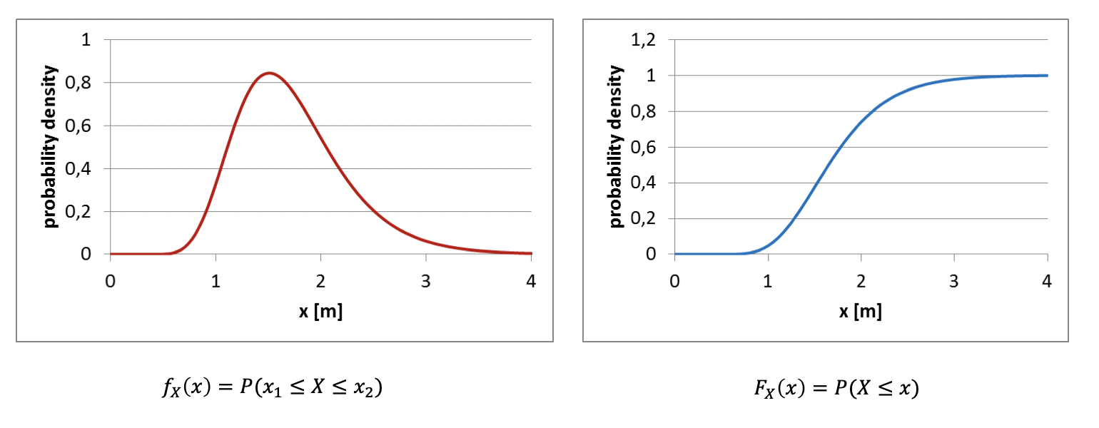
Different types of probability distributions exist and they can be derived based on the properties of the random process they shall describe. The normal distribution is just one of many and it results from processes that follow the central limit theorem.
The Normal Distribution has probability density and distribution as: $$ \begin{align} f_X(x)&=\frac{1}{\sigma_X\sqrt{2\pi}}e^{-0.5(\frac{x-\mu_X}{\sigma_X})} \label{_auto1}\\ F_X(x)&=\Phi\left(\frac{x-\mu_X}{\sigma_X}\right) \label{eq:NormDist} \end{align} $$\( \mu_X \) and \( \sigma_X \) are the mean value and the standard deviation of \( X \), and \( \Phi \) is the standard normal distribution function.
Although there are better distribution types for representing the timber bending strength \( f_{max,timber} \) and the snow load \( s \), we restrict our self to use the normal distribution for the sake of simplicity.
In order to assess the failure probability, the failure event has to be defined as a function of all the variables. In this example this means that failure \( F \) is defined as
$$ \begin{equation} F=\{M_{max, in}-M_{load,max} < 0\}=\{\frac{bh^2}{6}f_{max,timber}-\frac{s\cdot a\cdot l^2}{8} < 0\} \label{eq:failure} \end{equation} $$Limit State and Safety Margin: The term in the bracket above, i.e. that defines failure \( F \) is called a limit state and the so called general Safety Margin \( SM \) can be formulated as a difference between \( R \) the resistance and \( D \) the load effect (here \( R=M_{max, in} \) and \( D=M_{load,max} \)):
$$ \begin{equation} SM=R-D=\frac{bh^2}{6}f_{max,timber}-\frac{q_s l^2}{8} \label{eq:margin} \end{equation} $$Failure can be expressed as \( F=\{SM < 0\} \) and the failure probability as \( \Pr(F)=\Pr(SM < 0) \).
For the current example it is now seen that the failure probability can be straightforwardly computed if it is assumed that the snow load \( s \) and the timber strength \( f_{max,timber} \) can be represented as independent normal distributions with mean values \( \mu_{f_{max,timber}} \), \( \mu_{s} \) and standard deviations \( \sigma_{f_{max,timber}} \), \( \sigma_{s} \). Then the following general observations that nicely apply to this problem will help:
- If a random variable \( A \) has a mean value \( \mu_A \) and a standard deviation \( \sigma_A \), the random variable \( B=cA \) has a mean value \( c \mu_A \) and a standard deviation \( c \sigma_A \), where \( c \) is a constant.
- If \( X \) and \( Y \) are normal distributed random variables then \( Z=X+Y \) is also a normal distribution with a mean value \( \mu_Z=\mu_X+\mu_Y \) and a standard deviation \( \sigma_Z=\sqrt{ \sigma_X^2+\sigma_Y^2} \).
Applying 1):
$$ \begin{align} \mu_{R}&=\frac{bh^2}{6}\cdot \mu_{f_{max,timber}} \label{_auto2}\\ \sigma_{R}&=\frac{bh^2}{6}\cdot \sigma_{f_{max,timber}} \label{_auto3} \end{align} $$ $$ \begin{align} \mu_{D}&=\frac{a l^2}{8}\cdot \mu_{s} \label{_auto4}\\ \sigma_{D}&=\frac{a l^2}{8}\cdot \sigma_{s} \label{_auto5} \end{align} $$Applying 2):
Note that \( SM \) is normal distributed.
$$ \begin{align} \mu_{SM}&=\mu_{R}-\mu_{D} \label{_auto6}\\ \sigma_{SM}&=\sqrt{ \sigma_R^2+\sigma_D^2} \label{_auto7} \end{align} $$Failure Probability is then:
$$ \begin{align} \Pr(F)=\Pr(SM < 0)=F_M(0)&=\Phi\left(\frac{0-\mu_{SM}}{\sigma_{SM}}\right) \label{_auto8}\\ &=\Phi\left(-\frac{\mu_{R}-\mu_{D}}{\sqrt{ \sigma_R^2+\sigma_D^2}}\right) \label{_auto9} \end{align} $$Reliability Index: The reliability index is often used and is defined as:
$$ \begin{align} \beta=\frac{\mu_{R}-\mu_{D}}{\sqrt{\sigma_R^2+\sigma_D^2}} \label{_auto10} \end{align} $$such that
$$ \begin{align} \Pr(F)=\Phi\left(-\beta\right) \label{_auto11} \end{align} $$Lecture 8 - Excersises
Example - Rod loaded in tension 1
Consider the steel rod as illustrated in Figure 112. It is loaded by the force \( D \) and has yield stress of \( F_y \). The cross section area of the rod is \( A=10\; mm^2 \).
Figure 112: A steel rod that is loaded in tension.
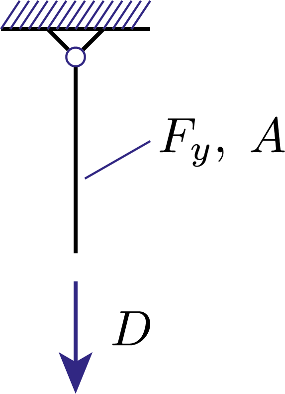
Both, the load \( D \) and the yield stress \( F_y \) are uncertain and represented by independent normal distributed random variables:
| Variable | Distribution | \( \mu \) | \( \sigma \) |
| \( D \) | Normal | 2 kN | 0.5 kN |
| \( F_y \) | Normal | 300 MPa | 30 MPa |
The probability of failure of the rod has to be computed.
Solution:
Resistance:
$$ \begin{align*} R=A\cdot F_y \; \Longrightarrow \; \mu_{R}&=A\cdot \mu_{F_y}= 300 \cdot 10 = 3\:kN \\ \sigma_{R}&=A\cdot \sigma_{F_y}=30 \cdot 10 = 0.3\:kN \end{align*} $$Safety margin \( M \) (in kN):
$$ \begin{align*} M=R-D \; \Longrightarrow \; \mu_{M}&=\mu_R-\mu_D= 3-2 = 1\:kN \\ \sigma_{M}&=\sqrt{\sigma_{R}^2+\sigma_{D}^2}= \sqrt{0.3^2+0.5^2} = 0.58\:kN \end{align*} $$Reliability index:
$$ \begin{align*} \beta=\frac{\mu_M}{\sigma_M}=\frac{1}{0.58}=1.71 \end{align*} $$Failure probability:
$$ \begin{align*} \Pr(F)=\Phi\left(-\beta \right)=4.36 \cdot 10^{-2} \end{align*} $$Note \( \Phi\left(x \right) \) can be obtained e.g. with a look up table.
End of Example - Rod loaded in tension 1.
Example - Rod loaded in tension 2
We consider the same rod with the same material property and loading as introduced above. This time we want to design the rod, i.e. choose the cross section area, such that it complies with a specified reliability criterion of \( \beta_{target}=4 \) or correspondingly \( \Pr(F)_{target}=3.17\cdot 10^{-5} \).
Solution:
$$ \begin{align*}A|:\; \beta \overset{!}{=} 4&= \frac{A\cdot \mu_{F_y}-\mu_D}{\sqrt{A^2\sigma_{F_y}^2+\sigma_D^2}}\\ \text{Solving for $A$:}\\ \Longrightarrow \; A&=\frac{\mu_{F_y}\mu_D+4\sqrt{\sigma_D^2\mu_{F_y}^2+\sigma_{F_y}^2\mu_{D}^2-16\sigma_{F_y}^2\sigma_D^2}}{\mu_{F_y}^2-16\sigma_{F_y}^2}=15.87\: mm^2 \end{align*} $$
End of Example - Rod loaded in tension 2.
Lecture 9 - Semi-Probabilistic Design concept
The computation of the failure probability and the reliability index can be demanding for practical routine structural design. It would be desirable to have design criteria that guarantee sufficient safety and at the same time do not require probabilistic analysis, i.e. only require deterministic calculus.
Considering one specific design case, it would be straight forward to set up a simple deterministic design concept by introducing a so called global safety factor \( SF \).
Example - Rod loaded in tension 3
Consider again the example with the steel rod from above. The reliability requirement was given as \( \beta_{target}=4 \) and we found out that \( A=15.87\: mm^2 \) did satisfy this safety requirement. Alternative to the reliability calculation we could also define a safety concept that is based on the mean values of the random variables and a global safety factor that is defined as
$$ \begin{align*} SF=\frac{15.87 \cdot \mu_{F_y}}{\mu_{D}}=2.38 \end{align*} $$End of Example - Rod loaded in tension 3.
More general for the problem \( M=R-D \) with normal distributed variables with known coefficients of variation \( cov_R \) and \( cov_D \), a direct correspondence between the global safety factor and the reliability index can be established:
$$ \begin{align*} \beta &= \frac{\mu_{R}-\mu_D}{\sqrt{\sigma_{R}^2+\sigma_D^2}}\\ \beta &= \frac{\mu_{R}-\mu_D}{\sqrt{\mu_{R}^2 cov_{R}^2+\mu_D^2 cov_D^2}}\\ \text{Introducing a global safety factor $\mu_{R}=SF\cdot \mu_D $:}\\ \beta &= \frac{SF\cdot \mu_D-\mu_D}{\sqrt{SF^2\cdot \mu_D^2 cov_{R}^2+\mu_D^2 cov_D^2}}\\ \beta &= \frac{SF-1}{\sqrt{SF^2 cov_{R}^2+ cov_D^2}}\\ \end{align*} $$A one-to-one correspondence between a global safety factor and a reliability requirement can be established for a specific case. However, this is not sufficient for a safety concept of a design code, where a large number of different designs situations has to be covered.
Partial factor safety concept
Design values:
As will be seen in an example later on, it is of advantage to put a safety factor on each variable in the limit state equation and introduce a design criterion based on so called design values of the corresponding variables.
We illustrate the concept again based on the simple problem \( M=R-D \) and the requirement:
$$ \begin{align*} \beta_{target} &\overset{!}{\leq} \frac{\mu_{R}-\mu_D}{\sqrt{\sigma_{R}^2+\sigma_D^2}}\\ \mu_{R}-\mu_D &\leq \beta_{target}\sqrt{\sigma_{R}^2+\sigma_D^2}\\ &\leq \beta_{target}\frac{\sigma_{R}^2+\sigma_D^2}{\sqrt{\sigma_{R}^2+\sigma_D^2}}\\ &\leq \beta_{target}\frac{\sigma_{R}}{\sqrt{\sigma_{R}^2+\sigma_D^2}}\sigma_{R}+\beta_{target}\frac{\sigma_D}{\sqrt{\sigma_{R}^2+\sigma_D^2}}\sigma_D\\ &\leq \beta_{target} \alpha_{R} \sigma_{R}+\beta_{target} \alpha_{D} \sigma_D\\ \end{align*} $$With \( \alpha_{R}=\frac{\sigma_{R}}{\sqrt{\sigma_{R}^2+\sigma_D^2}} \) and \( \alpha_{D}=\frac{\sigma_D}{\sqrt{\sigma_{R}^2+\sigma_D^2}} \).
Sorting \( R \)-parameters and \( D \)-parameters leads to
$$ \begin{align*} \mu_{R}-\beta_{target} \alpha_{R} \sigma_{R} &\leq \mu_D+\beta_{target} \alpha_{D} \sigma_D\\ \mu_{R}(1-\beta_{target} \alpha_{R} cov_{R}) &\leq \mu_D(1+\beta_{target} \alpha_{D} cov_D)\\ r_d&\leq d_d \end{align*} $$\( r_d \) and \( d_d \) are the so-called design values.
The design values are the values that should be used in the design in order to obtain a design solutions that complies with \( \beta_{target} \).
Example - Rod loaded in tension 4
For the rod example we obtain e.g.:
$$ \begin{align*} k=\sqrt{A^2\sigma_{F_y}^2+\sigma_D^2}=690.47\\ \alpha_{R}=\frac{A\sigma_{F_y}}{k}=0.69\\ \alpha_{D}=\frac{\sigma_{D}}{k}=0.72\\ \end{align*} $$ $$ \begin{align*} f_{y,d}=\mu_{F_y}-\beta_{target} \alpha_{F_y} \sigma_{R}=300-4 \cdot 0.69 \cdot 30 = 217.24\:MPa\\ d_{d}=\mu_{D}-\beta_{target} \alpha_{D} \sigma_{D}=2000+4 \cdot 0.72 \cdot 500 = 3448.28\:N\ \end{align*} $$Test:
$$ \begin{align*} r_d&\leq d_d\\ A \cdot f_{y,d}&\leq d_d\\ \Longrightarrow A &\leq \frac{d_d}{f_{y,d}}=\frac{3448.28}{217.24}=15.87\:mm \end{align*} $$End of Example - Rod loaded in tension 4.
Characteristic values:
In structural design codes as the Eurocodes, design values are obtained based on characteristic values. Characteristic values are defined as fractile or percentile values of the variables distribution functions. They are defined in the domain that is most significant for possible failure events, i.e. for variables that are related to the resistance, characteristic values are defined in the lower domain, for variables that are related to the load they are defined in the upper domain.
In the Eurocode the following general conventions are valid:
| Variable | Characteristic value |
| Material Resistance | 5%-Fractile |
| Variable Load | 98%-Fractile |
| Permanent Load | mean value |
In the following the equation for the design value and for the characteristic value for the normal sitribution are summarised. (generally for the random variable \( Y \))
Figure 113
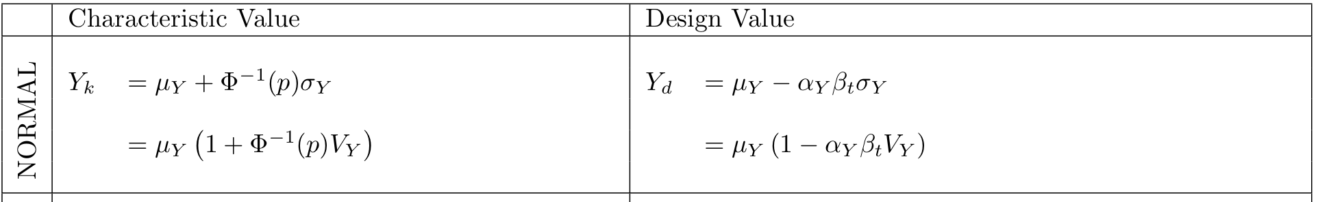
Note that \( \Phi^{-1}(0.05)=-1.64 \) and \( \Phi^{-1}(0.98)=2.05 \).
Partial safety factor: In order to compute the design value based on the characteristic value the so-called partial safety factor is introduced that is defined as:
For resistance variables \( R \):
$$ \begin{align} \gamma_R= \frac{\mu_R - \alpha_R\beta_t \sigma_R}{\mu_R + \Phi^{-1}(p) \sigma_R}=\frac{1- \alpha_R\beta_t cov_R}{1+ \Phi^{-1}(p) cov_R} \label{_auto12} \end{align} $$For resistance variables \( D \):
$$ \begin{align} \gamma_D= \frac{\mu_D + \Phi^{-1}(p) \sigma_D}{\mu_D + \alpha_D\beta_t \sigma_D}=\frac{1+ \Phi^{-1}(p) cov_D}{1+ \alpha_D\beta_t cov_D} \label{_auto13} \end{align} $$Example - Rod loaded in tension 5
For the rod example the characteristic values and the partial safety factors are computed as follows:
$$ \begin{align*} f_{y,k}=\mu_{F_y} + \Phi^{-1}(0.05) \sigma_{F_y}=300-1.64 \cdot 30 = 250.8 MPa \end{align*} $$ $$ \begin{align*} \gamma_{F_y} = \frac{f_{y,k}}{f_{y,d}} = \frac{250.8}{217.24} = 1.15 \end{align*} $$ $$ \begin{align*} d_{k}=\mu_{D} + \Phi^{-1}(0.98) \sigma_{D}=2000+2.05 \cdot 500 = 3025 MPa \end{align*} $$ $$ \begin{align*} \gamma_{D} = \frac{d_{d}}{d_{d}} = \frac{3448}{3025} = 1.14 \end{align*} $$End of Example - Rod loaded in tension 5.
Example - Beam with two loads
The simply supported beam in Figure 114 is to be designed for a specified target reliability index of \( \beta_t=4.2 \). The basic random variables that represent the situation are given below.
| Variable | \( G \) | \( Q^* \) | \( F_m \) |
| Mean (\( \mu_X \)) | 2 N/mm | 10000 N | 200 MPa |
| Standard dev. (\( \sigma_X \)) | 0.30 N/mm | 4000 N | 20 MPa |
| Coeff. of var. (\( COV_X \)) | 15% | 40% | 10% |
| Characteristic fractile (\( k_X \)) | 0.50 | 0.95 | 0.05 |
Figure 114: Beam geometry and loads.
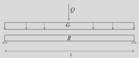
The limit state function for bending moment at mid-span is:
$$ \begin{align*} g(f_m,g,q)=W\cdot f_m-g\dfrac{l^2}{8}-q\dfrac{l}{4}\le 0 \end{align*} $$The corresponding reliability index is:
$$ \begin{align*} \beta = \dfrac{W\mu_{F_m}-\mu_G\dfrac{l^2}{8}-\mu_Q\dfrac{l}{4}}{\sqrt{\left(W\sigma_{F_m}\right)^2+\left(\sigma_G\dfrac{l^2}{8}\right)^2+\left(\sigma_Q\dfrac{l}{4}\right)^2}} \end{align*} $$Reliability based design:
The beam cross-section \( W \) can be chosen such that the reliability index of the beam corresponds to the target reliability, i.e. \( \beta=\beta_t \). This corresponds to the so-called reliability based design. E.g. for \( l=6 \) m, the section elastic modulus giving \( \beta=\beta_t \) is found to be \( W=3.01\cdot 10^5 \). The cross-section elastic modulus is plotted against the beam length in Figure 115.
Figure 115: Reliability based design for different beam lengths for \( \beta=\beta_t=4.2 \).
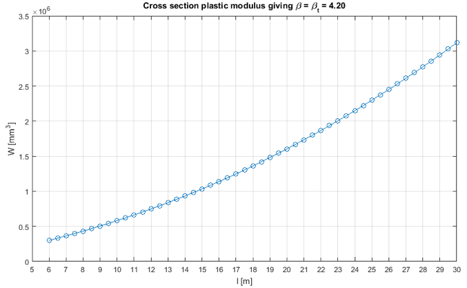
Partial factor design format: Although modern structural design codes (like Eurocodes) allow reliability based design, they propose simpler design procedures in the semi-probabilistic design format, where design equations are written in the load and resistance factor design format (LRFD). This format is referred to as semi-probabilistic, since random variables (represented by distribution functions) are reduced to design values, which are obtained from characteristic values as \( r_d=r_k/\gamma_R \) (for resistance) and \( s_d=s_k \cdot \gamma_S \) (for actions). The format is simpler, since the designer can check the design just by comparing design values, without the necessity of using reliability analyses. The design equation of the beam above is:
$$ \begin{align*} W\cdot f_{m,d}-g_d\dfrac{l^2}{8}-q_d\dfrac{l}{4}\le 0 \end{align*} $$where:
- \( f_{m,d}=\dfrac{f_{m,k}}{\gamma_R} \); \( g_{d}=g_k\gamma_G \) and \( q_{d}=q_k\gamma_Q \) are the \textbf{design values};
- \( f_{m,k}=F_{F_m}^{-1}(k_{F_m}) \); \( g_{k}=F_{G}^{-1}(k_{G}) \) and \( q_{k}=F_{Q}^{-1}(k_{Q}) \) are the \_characteristic values_ corresponding to the characteristic fractiles \( k_{F_m} \), \( k_{G} \) and \( k_{Q} \), which are defined arbitrarily and
- \( \gamma_G \); \( \gamma_R \) and \( \gamma_Q \) are the partial safety factors (p.s.f.).
The minimum cross-section plastic modulus satisfying the design equation is:
$$ \begin{align*} W_{min}=\dfrac{g_K\gamma_G \dfrac{l^2}{8}+q_K\gamma_Q \dfrac{l}{4}}{\dfrac{f_{m,k}}{\gamma_R}} \end{align*} $$Calibration of the partial factors for one given span (e.g. 6 m):
The p.s.f. need to be calibrated so that the design given with &W_{min}& fulfills a target safety. This corresponds to answer the question which values of the p.s.f. provide a design (i.e. \( W \)) associated with the reliability index \( \beta=\beta_t \)}?
The limit state function is rewritten with \( W=W_{min} \):
$$ \begin{align*} g(f_m,g,q)=\dfrac{g_K\gamma_G \dfrac{l^2}{8}+q_K\gamma_Q \dfrac{l}{4}}{\dfrac{f_{m,k}}{\gamma_R}}f_m-g\dfrac{l^2}{8}-q\dfrac{l}{4}\le 0 \end{align*} $$The beta index is evaluated correspondingly:
$$ \begin{align*} \beta = \dfrac{\left(\dfrac{g_K\gamma_G \dfrac{l^2}{8}+q_K\gamma_Q \dfrac{l}{4}}{\dfrac{f_{m,k}}{\gamma_R}}\right)\mu_{F_m}-\mu_G\dfrac{l^2}{8}-\mu_Q\dfrac{l}{4}}{\sqrt{\left(\left(\dfrac{g_K\gamma_G \dfrac{l^2}{8}+q_K\gamma_Q \dfrac{l}{4}}{\dfrac{f_{m,k}}{\gamma_R}}\right)\sigma_{F_m}\right)^2+\left(\sigma_G\dfrac{l^2}{8}\right)^2+\left(\sigma_Q\dfrac{l}{4}\right)^2}} \end{align*} $$where it is clear that the reliability of the design depends on the partial safety factors, i.e. \( \beta=\beta(\gamma_R,\gamma_G,\gamma_Q) \).
The partial safety factors are determined based on the sensitivity factors \( \alpha_{F_m},\alpha_G,\alpha_Q \):
$$ \begin{align*} \alpha_{F_m}&=\dfrac{-W\sigma_{F_m}}{k} \\ \alpha_{G}&=\dfrac{\left(\sigma_G\dfrac{l^2}{8}\right)}{k} \\ \alpha_{Q}&=\dfrac{\left(\sigma_Q\dfrac{l}{4}\right)}{k} \end{align*} $$Introducing \( W=3.01\cdot 10^5\:mm^3 \) that was found for \( l=6 \) m, the sensitivity factors are \( (\alpha_{F_m}=-0.699,\alpha_Q=0.698,\alpha_G=0.157) \). The corresponding partial safety factors are:
$$ \begin{equation} \begin{array}{l} \gamma_R^*=\dfrac{f_{m,k}}{f_{m,d}}=\dfrac{1+\Phi^{-1}(k_{F_m})\cdot COV_{F_m}}{1+\alpha_{F_m}\beta_t COV_{F_m}}=1.18\\ \\ \gamma_Q^*=\dfrac{q_{d}}{q_{k}}=\dfrac{1+\alpha_Q\beta_t\cdot COV_{Q}}{1+\Phi^{-1}(k_Q)COV_Q}=1.31\\ \\ \gamma_G^*=\dfrac{g_{d}}{g_{k}}=\dfrac{1+\alpha_G\beta_t\cdot COV_{G}}{1+\Phi^{-1}(k_G)COV_G}=1.10\\ \end{array} \label{_auto14} \end{equation} $$The calibrated p.s.f. obtained above result in a reliability \( \beta\ne\beta_t \), for a beam span \( l\ne 6 \) m, cf. Figure 116. This is due to the fact that the fraction of the external moment induced by \( G \) (or \( Q \)) changes with the beam span. The reliability for \( l=6 \) m is equal to the target, since that was the condition imposed for calibration. The reliability index is therefore dependent on the beam span (or equivalently the ratio between the moments induced by \( G \) and \( Q \)), i.e. \( \beta=\beta(\gamma_R,\gamma_G,\gamma_Q,l) \).
Figure 116: Reliability index of the beam designed with p.s.f optimized for \( l=6 \) m.
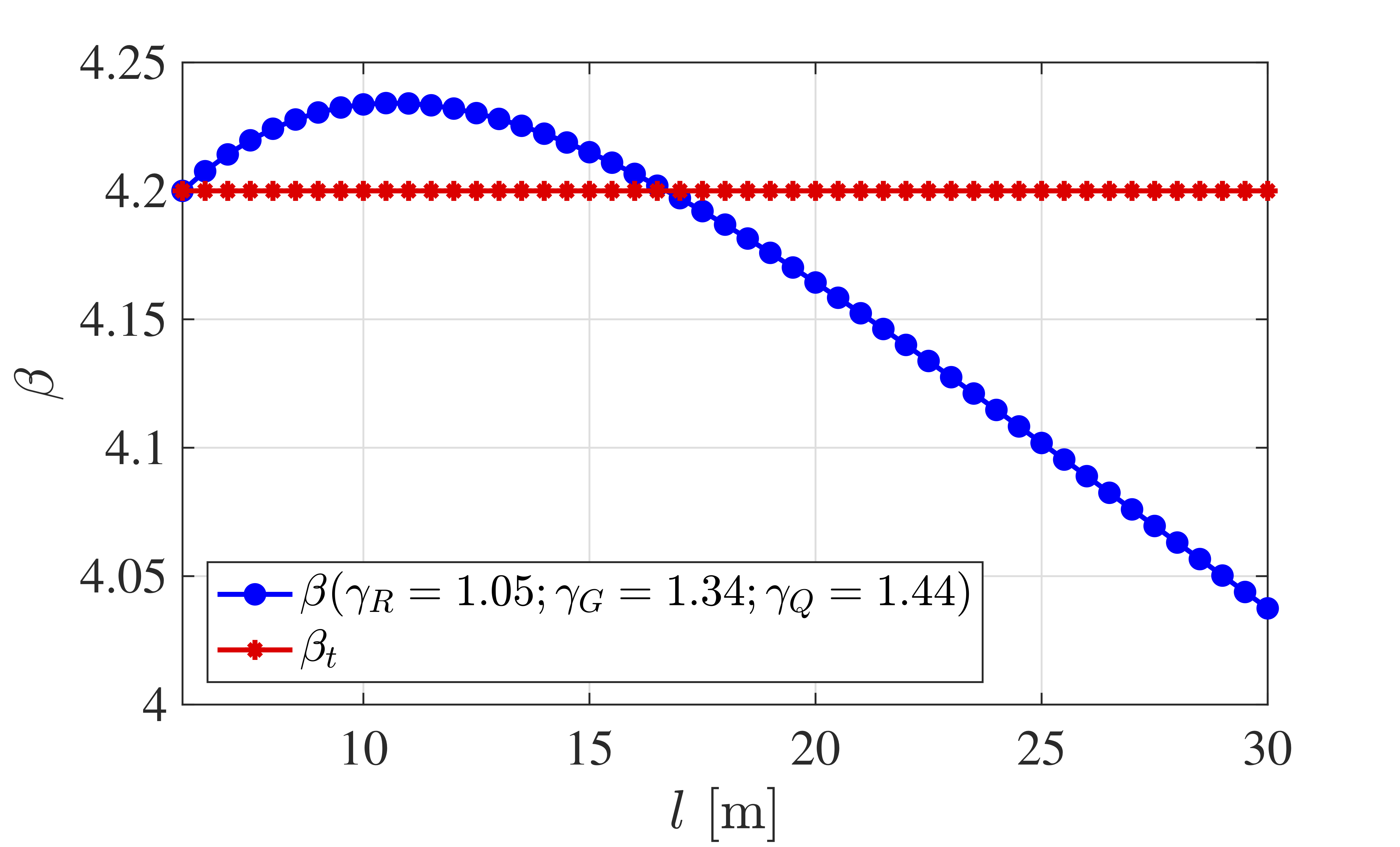
In order to get a constant reliability, i.e. independent of the geometry, a new set of p.s.f should be calibrated for each beam length, see Figure 117.
Figure 117: Reliability index of the beam designed with p.s.f optimized for \( l=6 \) m.
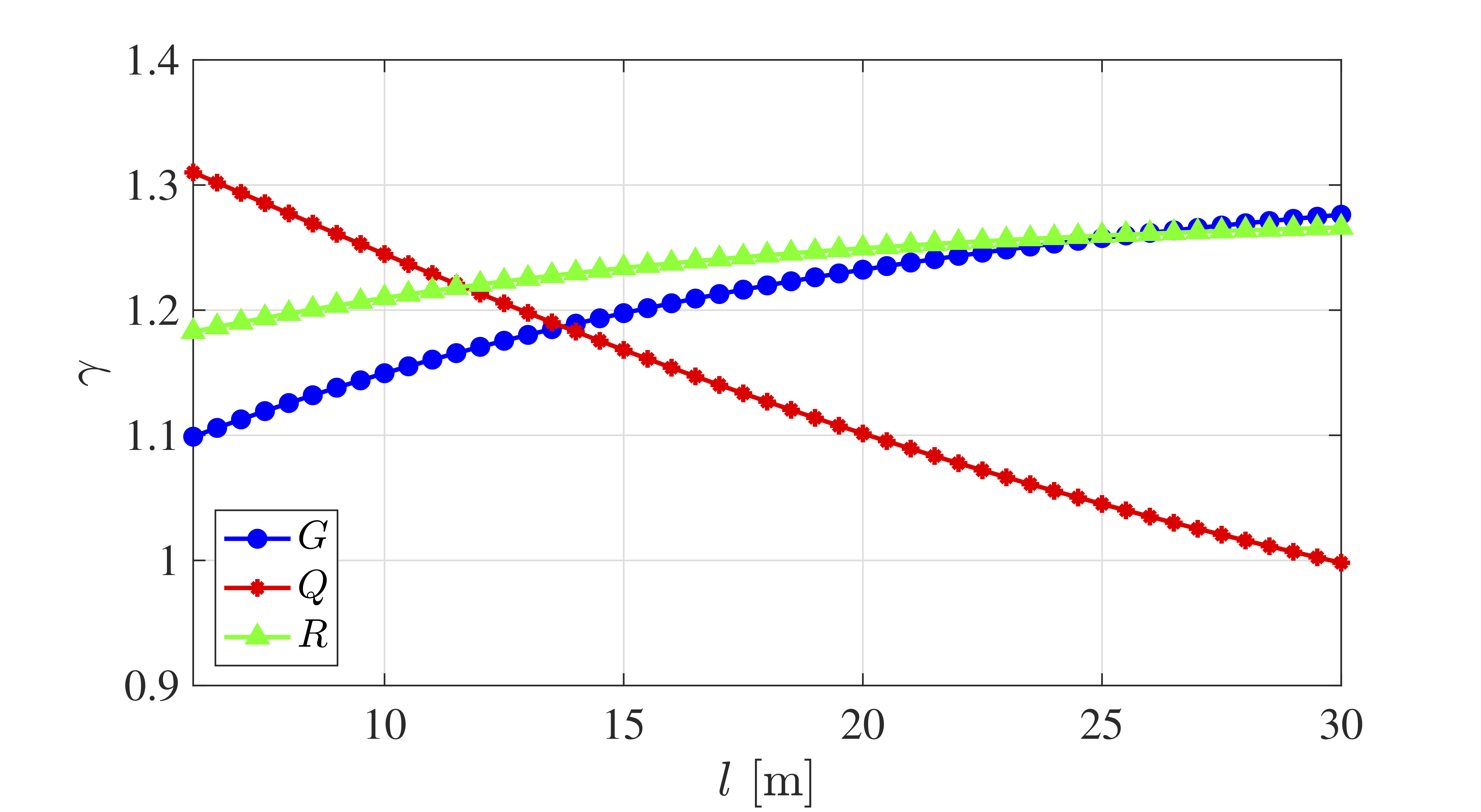
This is not practical and not implemented in design codes. The problem is solved by finding the set of p.s.f which ensures the reliability to be as homogeneous as possible over a range of possible scenarios. This set can be obtained by solving the minimization problem:
$$ \begin{align*} \min_{\gamma_R^*,\gamma_G^*,\gamma_Q^*}\left\{ {\sum}_{i=1}^n\left(\beta_t-\beta_i(\gamma_R,\gamma_G,\gamma_Q,l_i)\right)^2\right\} \end{align*} $$The set of p.s.f obtained is \( (\gamma_R^*=1.08,\gamma_G^*=1.38,\gamma_Q^*=1.35) \). The corresponding reliability is plotted in Figure 118.
Figure 118: Reliability index of the beam designed with p.s.f optimized for \( l=6 \) m.
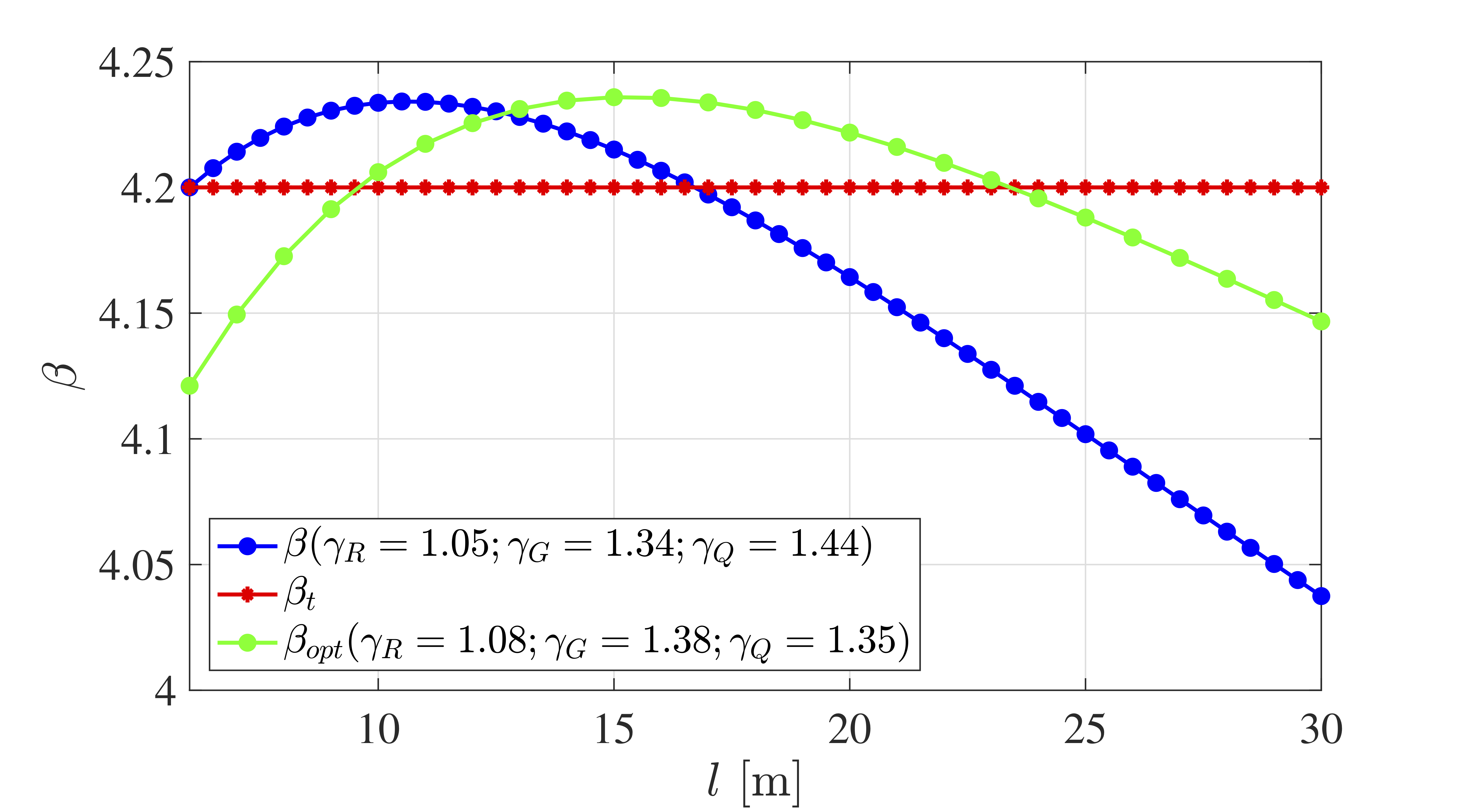
Global Safety Factor: An alternative (and older) format of semi-probabilistic design equations makes use of the global safety factor (\( SF \)). The design equation with the global safety factor applied on the mean values reads:
$$ \begin{align*} \dfrac{W\mu_{F_m}}{\mu_G\dfrac{l^2}{8}+\mu_Q\dfrac{l}{4}}>SF \end{align*} $$where the numerator is the mean value of the moment resistance and the denominator is the mean value of the action induced moment.
As before, \( SF \) can be calibrated so that the design equation provides a design with the target level of risk. The limit state function is rewritten with \( W= W_{min} \):
$$ \begin{equation*} g(f_m,g,q)=\dfrac{SF}{\mu_{F_m}}\left(\mu_G\dfrac{l^2}{8}+\mu_Q\dfrac{l}{4}\right)\cdot f_m-g\dfrac{l^2}{8}-q\dfrac{l}{4}\le 0 \end{equation*} $$Consequently the reliability index \( \beta \) is evaluated as:
$$ \begin{equation*} \beta = \dfrac{\dfrac{SF}{\mu_{F_m}}\left(\mu_G\dfrac{l^2}{8}+\mu_Q\dfrac{l}{4}\right)\mu_{F_m}-\mu_G\dfrac{l^2}{8}-\mu_Q\dfrac{l}{4}}{\sqrt{\left(\dfrac{SF}{\mu_{F_m}}\left(\mu_G\dfrac{l^2}{8}+\mu_Q\dfrac{l}{4}\right)\sigma_{F_m}\right)^2+\left(\sigma_G\dfrac{l^2}{8}\right)^2+\left(\sigma_Q\dfrac{l}{4}\right)^2}} \end{equation*} $$where it is clear that the reliability of the design is depending on the global safety factor, i.e. \( \beta=\beta(SF) \).
The global safety factor is calibrated by setting \( \beta(SF)\equiv \beta_t \). As an example, considering \( l=6 \) m, the calibrated global safety factor is found with numerical minimisation to be \( SF^*=2.51 \), giving \( W=300610 \) mm \( ^3 \).
As before, the design performed with the calibrated \( SF \) for \( l=6 \) m results in a different reliability for different spans. The \( SF \) can be calibrated so to give a reliability as homogeneous as possible over the different design scenarios. Therefore, as previously, the \( SF \) can be calibrated by solving a minimization problem.
$$ \begin{equation*} \min_{SF^*}\left\{ {\sum}_{i=1}^n\left(\beta_t-\beta_i(SF^*,l_i)\right)^2\right\} \end{equation*} $$The optimized \( SF \) obtained is \( SF^*=2.20 \), see Figure 119.
Figure 119: Reliability index for \( SF \) calibrated for \( l = 6 \) m (in blue) and for different scenarios simultaneously (in green).
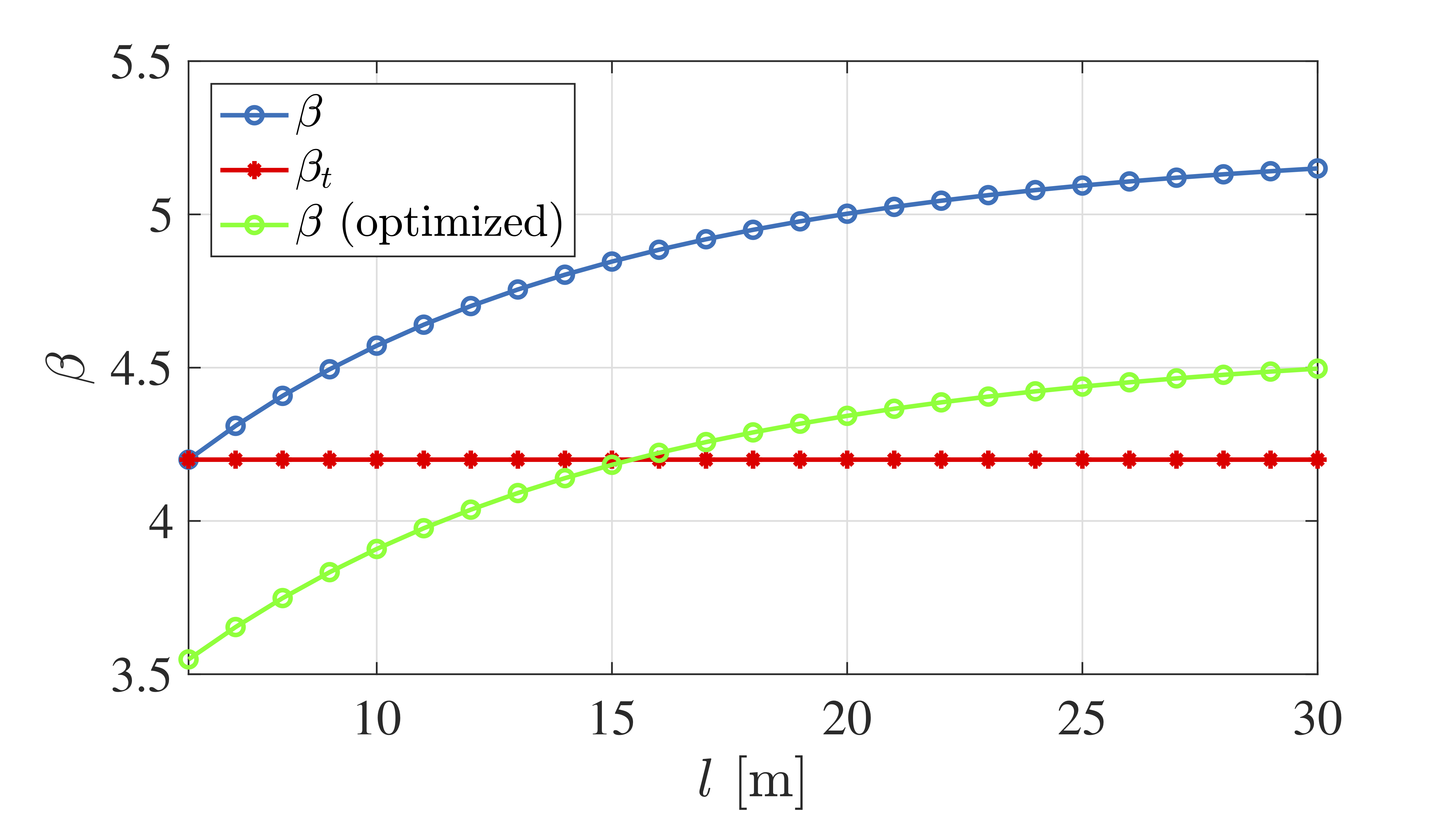
Comments and observations:
It can be observed from Figure 118 and Figure 119 that, by changing the \( SF \) the curve is only shifted up and down while the three p.s.f. shift and distort the curve (note that the vertical axes of both figures have different scale). This leads to higher levels of optimization (i.e. a flatter curve) with p.s.f.. The values of \( \sum_{i=1}^n\left(\beta_t-\beta_i\right)^2 \) show clearly this differences in the two formats. In fact, after optimization \( \sum_{i=1}^n\left(\beta_t-\beta_i\right)^2=0.026 \) for the p.s.f. format and \( \sum_{i=1}^n\left(\beta_t-\beta_i\right)^2=1.88 \) for the global safety factor format. The load and resistance factor design method offers therefore a more homogenized level of safety.
Figure 120: Comparison of \( \beta \) values for \( SF \) and partial safety factors (LRFD) formats before and after optimisation.
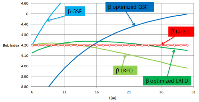
Lecture 10 - Semi-Probabilistic Design according to the EUROCODES
The learning goal of today is:
- develop basic competence in applying the load combination rules of the EUROCODES
Reading / Homework:
- This lecture notes
- Get basic orientation about EN 1990
- Designers' guide to Eurocode 0
Principles
In the Eurocodes a semi-probabilistic design method is introduced through partial factor design that should generally be applied as default design method for common design situations. The partial factor design format is formulated such that it facilitates the identification of acceptable and feasible design solutions concerning new structures. The partial factor design format comprises:
- consequence class categorization (see EN1990 Annex B);
- design situations (see ENs 1990 to 1999);
- design equations (see ENs 1990 to 1999);
- design values (as determined according EN1990, section 6).
Design equations can be formulated for failure of individual cross sections of a structure or for failure of several cross sections and/or components.
Implementation
The principle form of the design equation is given as
$$ \begin{align} R_d-E_d\geq 0 \label{eq:design} \end{align} $$, where \( R_d \) is the design value for the load bearing capacity and \( E_d \) is the design value for the action effect.
The design value of a basic variable \( Y \) is defined as the multiplication or division of a corresponding partial safety factor \( \gamma_Y \) and the characteristic value \( Y_k \). Accordingly, Equation \eqref{eq:design} can be written as
$$ \begin{align} \frac{R_k}{\gamma_R}=R_d>E_d=\gamma_E E_k \label{eq:design2} \end{align} $$The characteristic value \( Y_k \) is taken as a specified \( p- \) fractile value from the statistical distribution \( F_Y \) that is chosen to represent the basic variable, as
$$ \begin{align} Y_k=F_{Y}^{-1}(p) \label{eq:char} \end{align} $$where \( F_Y \) is the cumulative probability distribution function of the basic variable \( Y \).
Typical values for \( p \) are:
- resistance related variables: \( p=0.05 \);
- permanent actions: \( p=0.5 \);
- time-variable actions: \( p=0.98 \) (referring to the distribution of the yearly extreme values).
Load Combination
The design value for the action effect \( E_d \) is generally obtained by combining action effects from different sources that are relevant for the structure at hand. Each critical cross section is thereby considered separately and the largest load effect taken from different combination options is taken as relevant.
When combining action effects it is distinguished between permanent actions \( G_j \) and variable actions \( Q_i \).
For variable actions the so-called load combination factor \( \psi_0 \) is introduced that takes into account that extremes of variable actions do not happen simultaneously.
Load combination factors for different variable actions are given in EN1990, Table NA.A1.1:
Figure 121
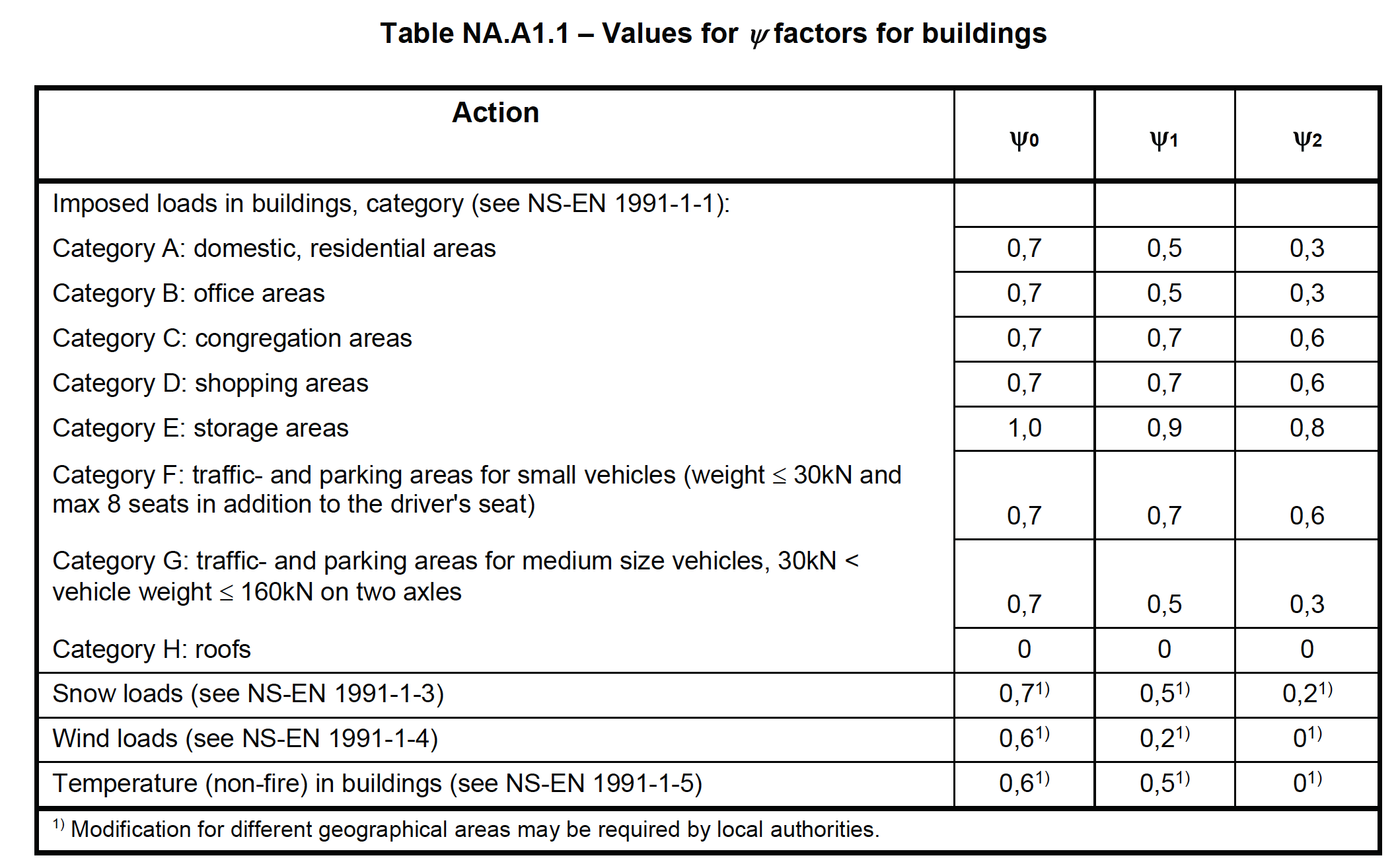
The load combination rules and the specification of the partial safety factors for permanent and variable load effects are then given in EN 1990 Table NA.A1.2(B):
Figure 122
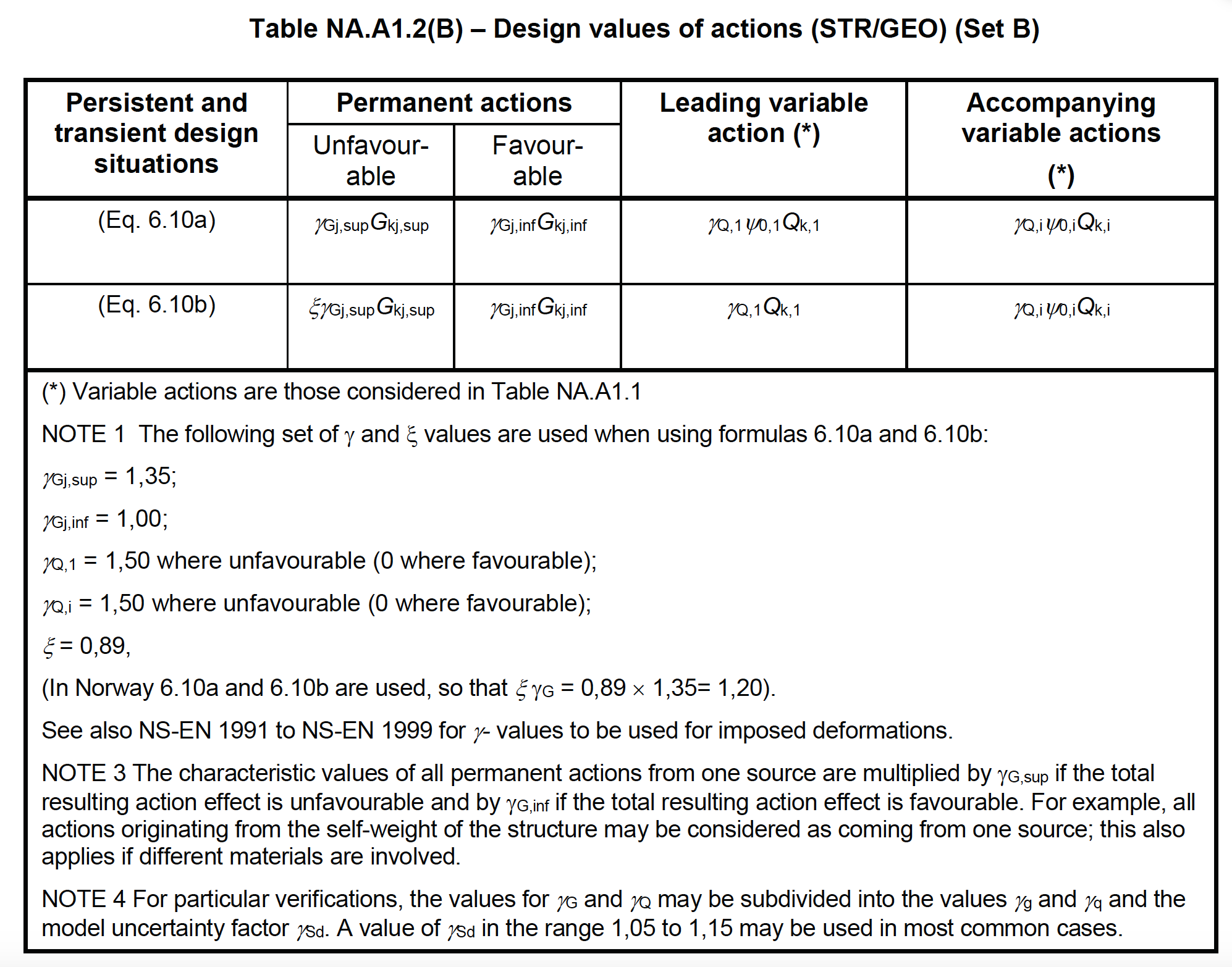
The table specifies partial factors for actions with favorable and unfavourable effect. It also distinguishes situations where the permanent load is dominant (Eq.6.10a) and where one of the variable loads is dominant (Eq.6.10a). Correspondingly for a load combination problem with \( n \) (unfavourable) variable loads, \( n+1 \) load combinations have to be evaluated, whereas the one that gives the largest absolute load effect is considered as the relevant.
Example 1
(Solution by Jorge Espinosa Mendoza)Figure 123
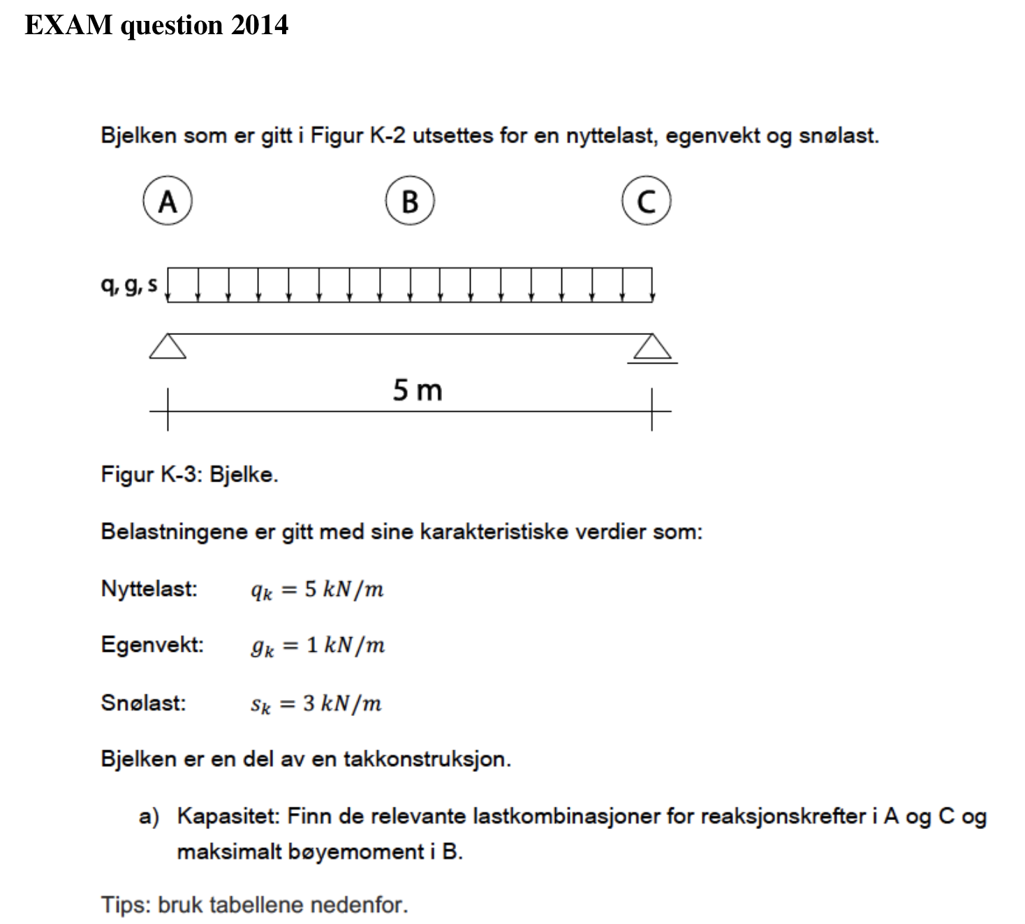
Solution:
The combination of actions for an ultimate limit state is covered in the Chapter 6 of NS EN 1990:2002. Given the characteristic values of the acting loads, the design value of the individual actions and their combined effect is to be assessed. It is assumed that the clause 6.1(2) is satisfied, i.e. 'Actions that cannot occur simultaneously, for example due to physical reasons, should not be considered together in combination’.
Permanent, variable and accidental loads are to be combined. Permanent actions that yield unfavourable effects are given by their upper design values. Permanent actions that yield favourable effects are given by their lower design values. Variable actions are categorized as either leading or accompanying actions. The leading action is to be assessed with its characteristic value \( Q_{k,1} \). The combination value \( \psi_{0,i} Q_{k,i} \) is to be used for the accompanying actions. When it is not trivial to identify this categorization, each variable is to be sequentially considered as the leading one.
For the ultimate limit states, NS EN 1990:2002 allows to use the less favourable of the expressions in Eqs. (6.10a) and (6.10b). In Eq. (6.10a), all the variable actions are assumed to be accompanying actions, i.e. the combination value is used for all the variable actions. In Eq. (6.10b), one variable action is identified as the leading action and a reduction factor \( \xi \) is applied to the unfavourable permanent actions (\( \xi = 0.89 \)). Generally speaking, it might be needed to try different combinations of leading and accompanying variable loads to find out what is the most unfavourable combination.
In this example, the loads are all unfavourable regarding reactions in A and C and bending moment in B. The design load is calculated according to Eqs. (6.10a) and (6.10b) below.
Application of 6.10a:
According to Table NA.A1.1 of Norwegian National Annex of NS EN 1990:2002, \( \psi_0=0 \) for imposed loads in roofs and \( \psi_0=0.7 \) for snow loading (in Norway).
$$\begin{array}{l} \gamma_{G,sup}g_k+\gamma_{Q,1}\psi_{0,1}q_{k,1}+\gamma_{Q,2}\psi_{0,2}s_{k,2}\\ \\ =1.35\cdot 1 \dfrac{\text{kN}}{\text{m}}+1.50\cdot 0\cdot 5\dfrac{\text{kN}}{\text{m}}+1.50\cdot 0.7\cdot 3\dfrac{\text{kN}}{\text{m}}\\ \\ =4.5\dfrac{\text{kN}}{\text{m}} \end{array}$$Application of 6.10b:
Since there are two variable actions, two load combinations are tested in order to find the design load combination. First, it is assumed that the life-load (nyttelast) is leading and afterwards, the case with the snow load (snølast) leading is assessed.
\( Q \) leading:
$$\begin{array}{l} \xi\gamma_{G,sup}g_k+\gamma_{Q,1}q_{k,1}+\gamma_{Q,2}\psi_{0,2}s_{k,2}\\ \\ =0.89\cdot 1.35\cdot 1 \dfrac{\text{kN}}{\text{m}}+1.50\cdot 5\dfrac{\text{kN}}{\text{m}}+1.50\cdot 0.7\cdot 3\dfrac{\text{kN}}{\text{m}}\\ \\ =11.85\dfrac{\text{kN}}{\text{m}} \end{array}$$
\( S \) leading:
$$\begin{array}{l} \xi\gamma_{G,sup}g_k+\gamma_{Q,1}s_{k,1}+\gamma_{Q,2}\psi_{0,2}q_{k,2}\\ \\ =0.89\cdot 1.35\cdot 1 \dfrac{\text{kN}}{\text{m}}+1.50\cdot 3\dfrac{\text{kN}}{\text{m}}+1.50\cdot 0\cdot 5\dfrac{\text{kN}}{\text{m}}\\ \\ =5.70\dfrac{\text{kN}}{\text{m}} \end{array}$$
Therefore, the design load for the reactions at A and B and moment at B is \( 11.85 kN/m \), given by Eq. 6.10b with the life-load \( Q \) leading.
Equilibrium limit state
So far we have introduced the procedure for combining loads for ultimate limit states where the failure/rupture of a cross section is the event of interest. The limit state is the formulated by comparing the combined load with the load bearing resistance of the considered cross section.
A situation that often also becomes relevant is the so-called equilibrium limit state. Here, the loss of static equilibrium is represented by the limit state. The corresponding load combination rules are found in EN 1990 Table NA.A1.2(A):
Figure 124
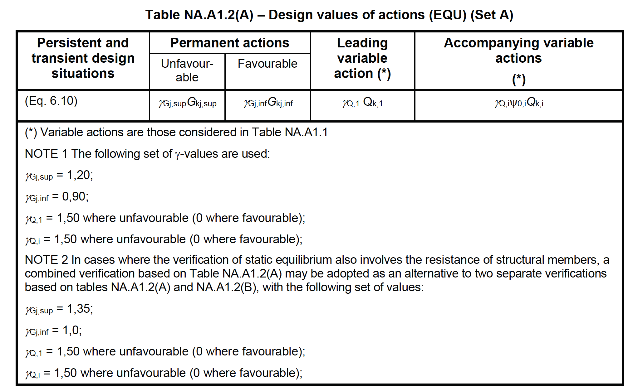
Example 2
(Example developed by Jorge Espinosa Mendoza)Consider the beam in Figure 125 loaded with the self-weight \( G \) and the variable life-load \( Q \). The beam is part of a balcony in a residential building.
Figure 125: Simple supported beam with cantilever arm. .
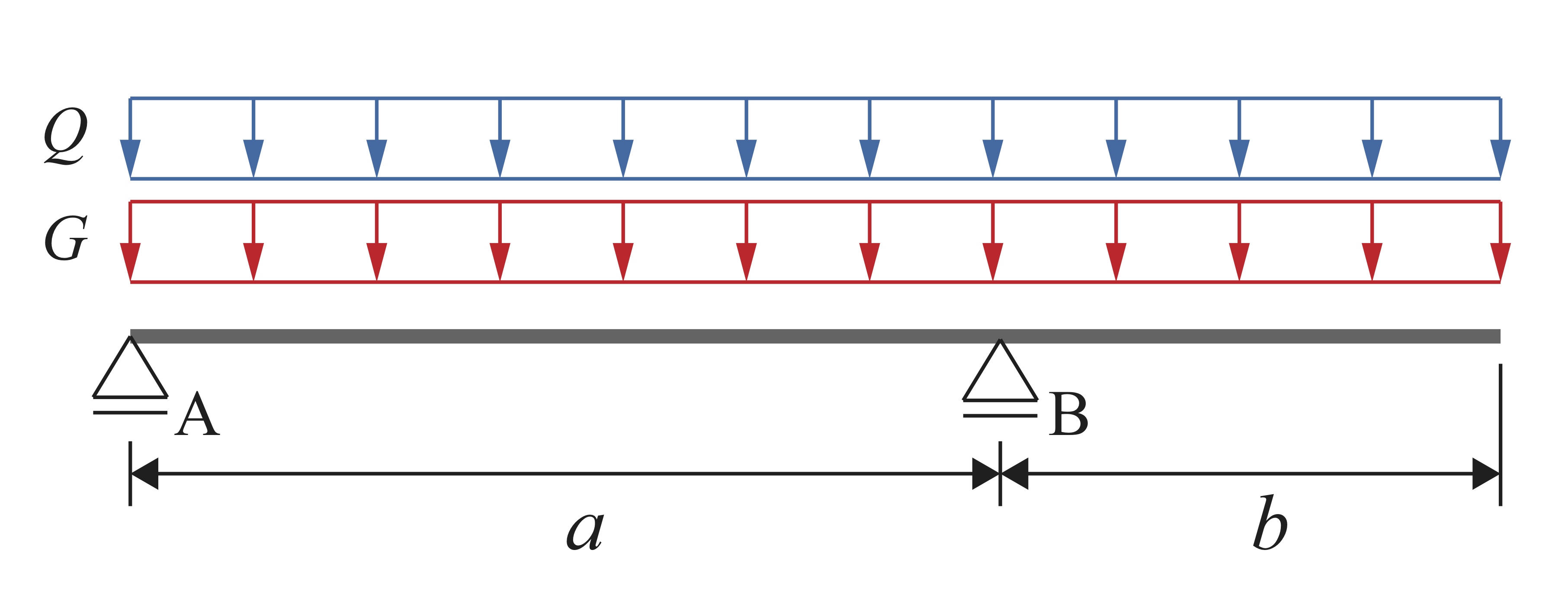
The characteristic values of the actions are \( g_k=2 \) kN/m; \( q_k=4 \) kN/m.
1. What is the maximum ratio \( b/a \) that verifies the equilibrium limit state? Assume that the supports cannot provide tension reactions.
Figure 126
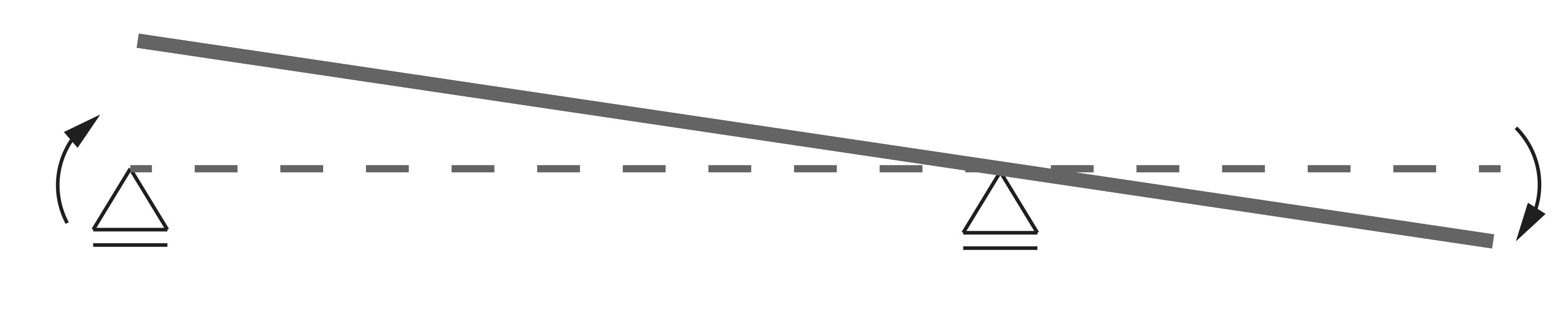
2. Consider \( a=10 \) m and \( b=4.6 \) m. Calculate the design bending moment \( M_{ED} \) acting on the beam.
Solution
1:
The verification of the limit states implies that design's probability of not satisfying them is small enough. According to NS EN 1990:2002, the following limit states are to be considered for the design of a structure:
a) EQU: Loss of static equilibrium of the structure or any part of it considered as a rigid body, where:
- minor variations in the value or the spatial distribution of actions from a single source are
significant, and
- the strengths of construction materials or ground are generally not governing;
b) STR: Internal failure or excessive deformation of the structure or structural members, including footings, piles, basement walls, etc., where the strength of construction materials of the structure governs;
c) GEO: Failure or excessive deformation of the ground where the strength of soil or rock are significant in providing resistance;
d) FAT: Fatigue failure of the structure or structural members.
Clause 6.4.3.1(4)P is to be considered for the load combination of an EQU limit state: Where the results of a verification may be very sensitive to variations of the magnitude of a permanent action from place to place in the structure, the unfavourable and the favourable parts of this action shall be considered as individual actions.
Therefore, the loads can be divided to consider their design values under the favourable or unfavourable assumptions. Taking this into account, the acting loads are divided as in EN 1990 Table NA.A1.2(A), where the \( \gamma \)-factors are given for equilibrium design value actions.
Figure 127: Load combination for the EQU limit state. .
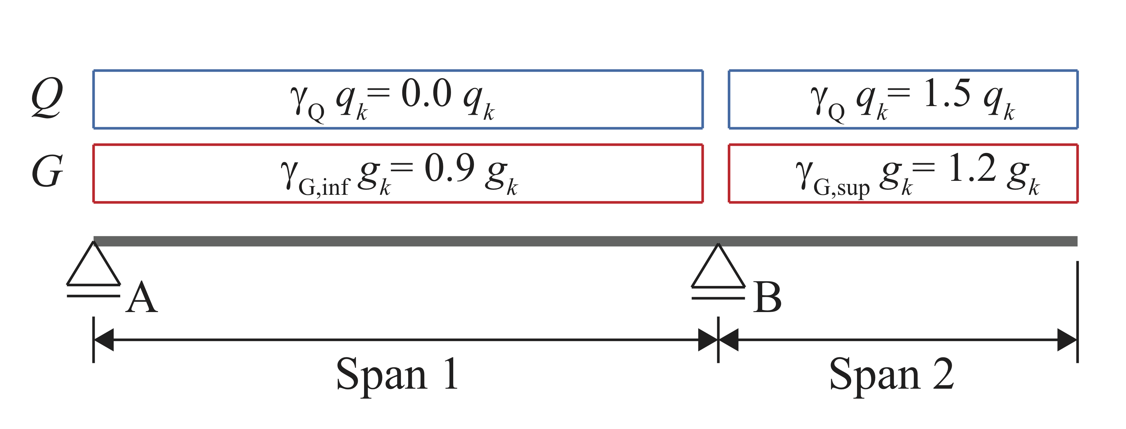
The characteristic values of the self-weight \( G \) and the imposed load \( Q \) are \( g_k=2 \) kN/m and \( q_k=4 \) kN/m, respectively. The design load is then calculated separately for both spans:
Span 1: $$ \begin{align*} q_a=\gamma_{G,inf}g_k+\gamma_Q q_k=0.9\cdot 2+0\cdot 4=1.8\; kN/m \end{align*} $$ Span 2: $$ \begin{align*} q_b=\gamma_{G,sup}g_k+\gamma_Q q_k=1.2\cdot 2+1.5\cdot 4=8.4\;kN/m \end{align*} $$Figure 128: Loads acting for the EQU limit state.
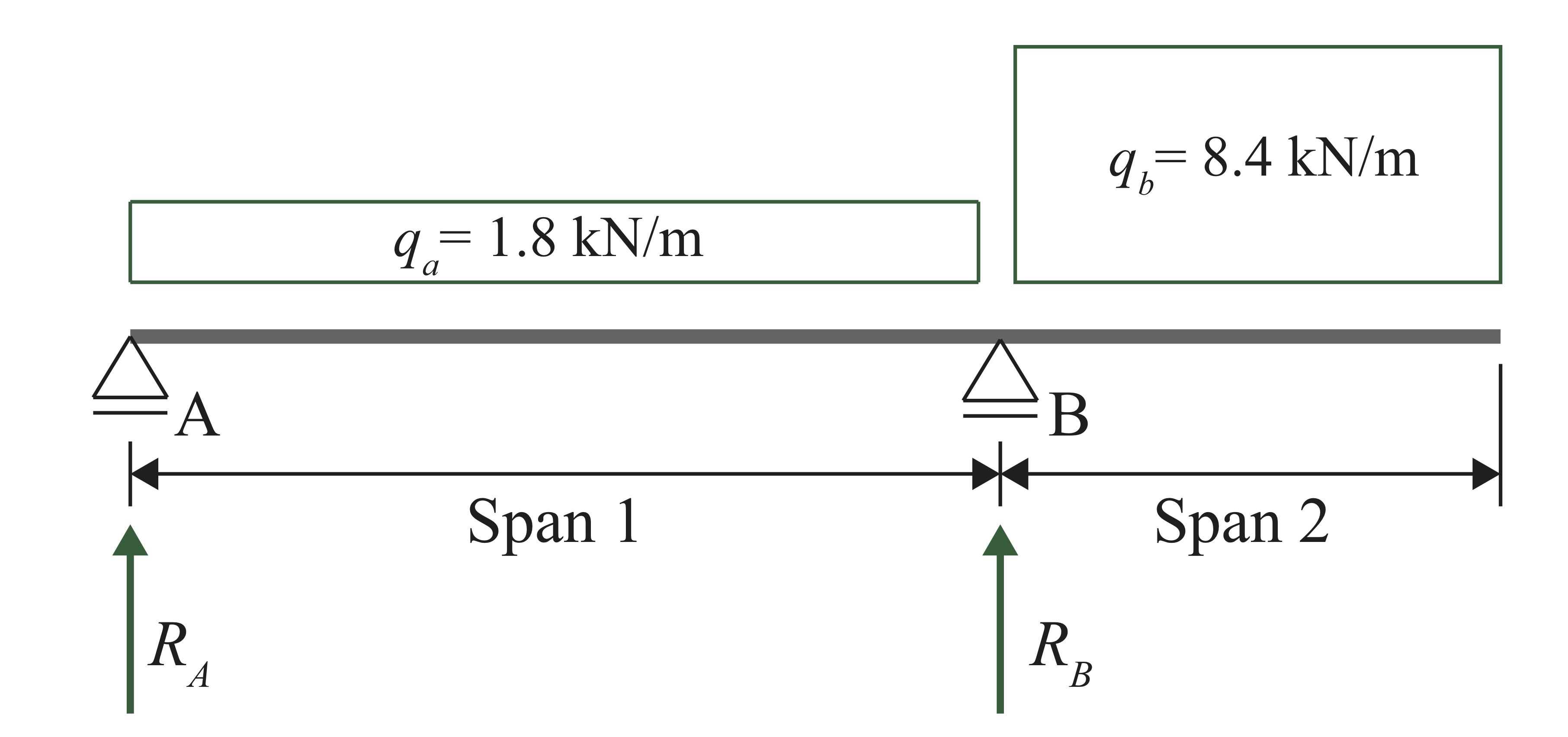
The equilibrium is to be checked with the load configuration in Figure 128, taking into account that the supports do not take any upward force. Mathematically, this translates to: equilibrium is not verified when the reaction at the support A is negative. The reactions at the supports A and B are directly determined by the equilibrium of forces and moments.
Equilibrium of moments around B: $$ \begin{align} q_b \dfrac{b^2}{2}+R_A a -q_a\dfrac{a^2}{2}=0 \rightarrow R_A=q_a\dfrac{a}{2}-q_b\dfrac{b^2}{2a} \label{eq:eq1} \end{align} $$ Equilibrium of forces: $$ \begin{align} R_A+R_B-q_a\cdot a-q_b\cdot b=0 \rightarrow R_B=q_a\cdot a+q_b\cdot b-R_A \label{_auto15} \end{align} $$A parameter \( k\in \rm I\!R^+ \) is introduced, defined as \( k=b/a \). Given the design loads, the equilibrium is verified depending on \( k \). The case in which the EQU limit state is just verified is related to a ratio \( k=k_{lim} \). When the cantilever span \( b \) becomes longer than a limit value (\( b\geq k_{lim}a \)), equilibrium is only satisfied with a negative value of \( R_A \), i.e. holding the beam down at the support A.
The load effects, i.e. the shear forces and bending moments along the beam, are computed applying equilibrium with the external actions. In Figure 129 (a) and (b), the shear and bending diagrams are illustrated for \( k < k_{lim} \) and \( k=k_{lim} \), respectively.
Figure 129: Loads acting for the EQU limit state.
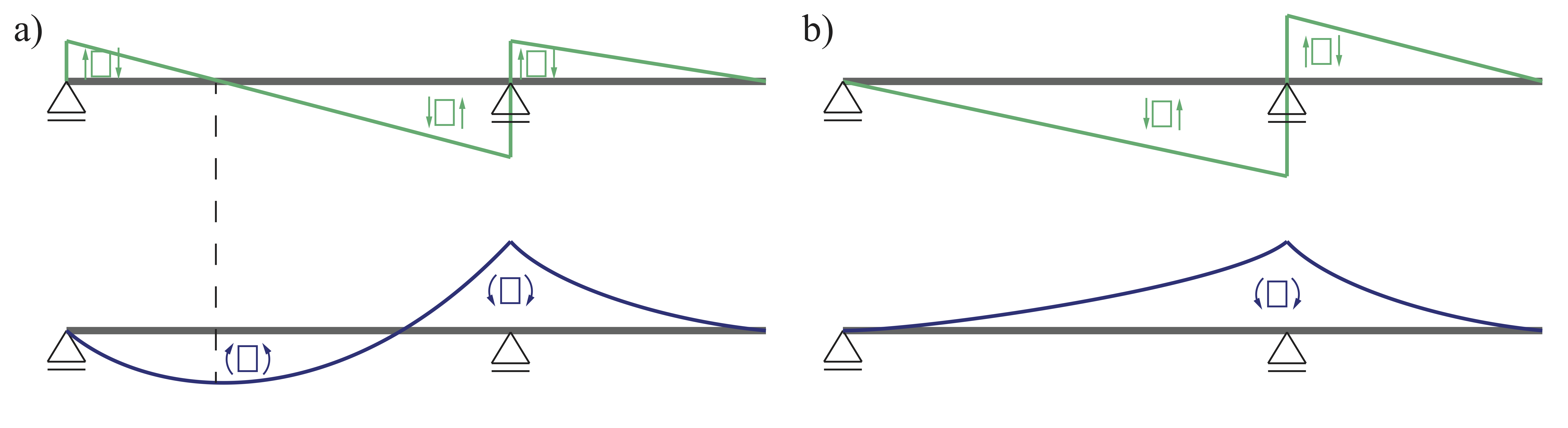
Substituting \( b=ka \) in Eq.\eqref{eq:eq1} results in:
$$ \begin{align*} R_A=q_a\dfrac{a}{2}-q_b\dfrac{k^2a}{2} \end{align*} $$Setting \( R_A=0 \) yields:
$$ \begin{align*} R_A=0=q_a\dfrac{a}{2}-q_b\dfrac{k_{lim}^2a}{2} \end{align*} $$Now is direct to isolate \( k_{lim} \) to just satisfy the EQU limit state:
$$ \begin{align*} k_{lim}=\sqrt{q_a\dfrac{a}{2}-\dfrac{2}{q_b a}}=\sqrt{\dfrac{q_a}{q_b}}=\sqrt{\dfrac{1.8}{8.4}}=0.46 \end{align*} $$Therefore, \( b \) must be less or equal than \( 0.46a \) in order to satisfy EQU. In Figure 130, it can be observed the relation between the reaction at the support A and \( k \).
Figure 130: Parameter study.
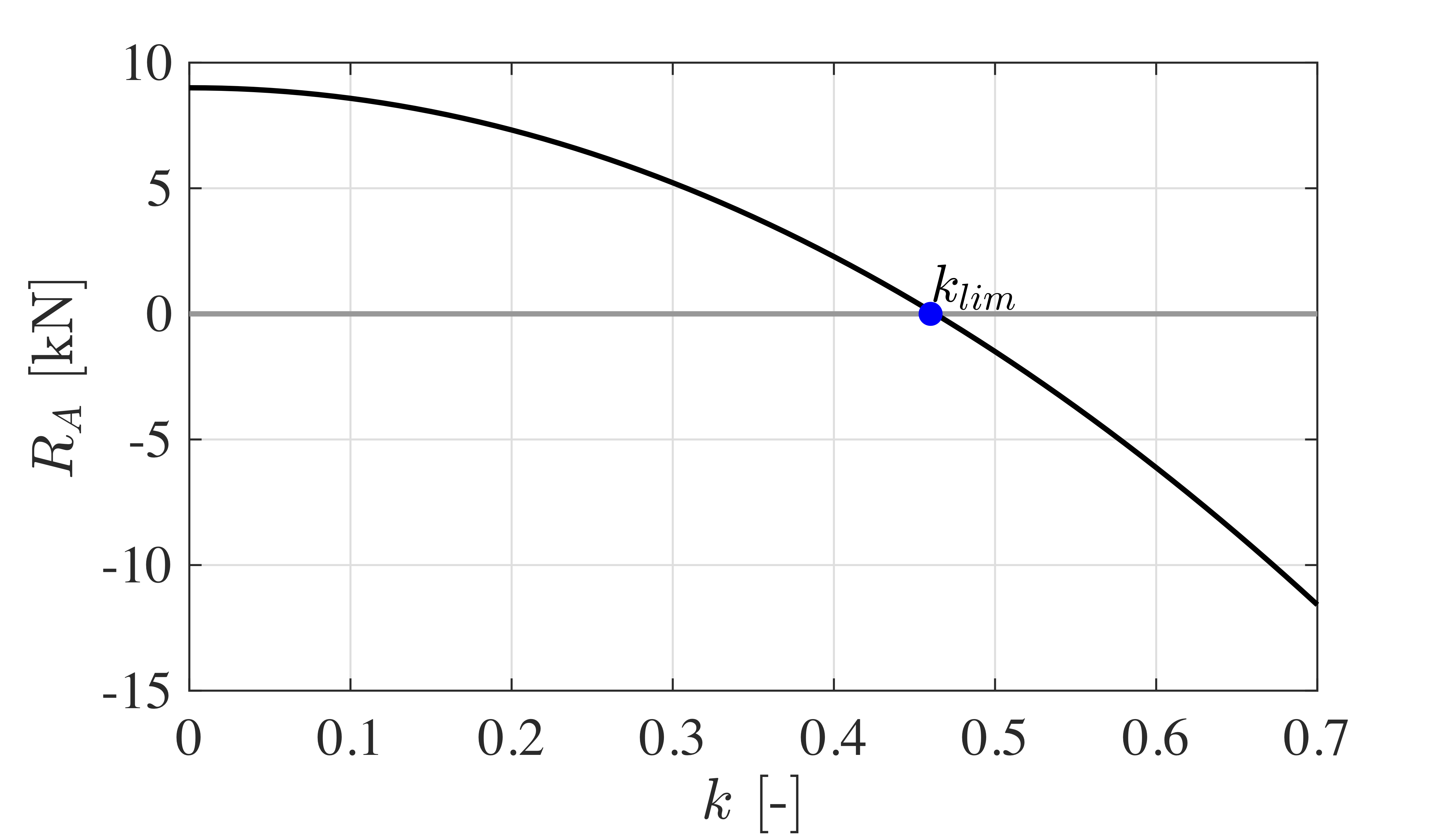
2:
Setting \( a=10 \) m and \( b=4.6 \) m the EQU limit state is verified. The bending moment at the support B results in:
$$ \begin{align*} M_{B}=q_b \dfrac{b^2}{2}=-8.4\dfrac{4.6^2}{2}= -89.2 \text{kNm} \end{align*} $$In order to calculate the design moment \( M_{Ed} \), the STR limit state is to be verified as well. The maximum negative and positive bending moments occur at the support B and at an intermediate point C of the Span 1, respectively. \( M_{Ed} \) is the maximum (in absolute value) between both. The design loads of the STR limit state differ from the ones used for the EQU verification. Table NA.A1.2(B) applies for the verification of the STR limit state.
The following should be noticed: Note 3 in Table (NA)A1.2(B) of (NS)EN 1990:2002: The characteristic values of all permanent actions from one source are multiplied by \( \gamma_{G,sup} \) if the total resulting action effect is unfavourable and \( \gamma_{G,inf} \) if the total resulting action effect is favourable. For example, all actions originating from the self weight of the structure may be considered as coming from one source; this also applies if different materials are involved.
Bending moment in B: \( q_a \) and \( q_b \) UNFAVOURABLE.
Eq.(6.10a) of NS EN 1990:2002 $$ \begin{array}{l} q_{a,d}=\gamma_{G,sup}g_k+\psi_{0,Q}\cdot\gamma_Q \cdot q_k=1.35\cdot 2+0.7\cdot 1.5\cdot 4=6.9 \text{kN}/\text{m}\\ q_{b,d}=q_{a,d} \end{array} $$ Eq.(6.10b) of NS EN 1990:2002 $$ \begin{array}{l} q_{a,d}=\xi\gamma_{G,sup}g_k+\gamma_Q q_k=0.89\cdot 1.35\cdot 2+1.5\cdot 4=8.3 \text{kN}/\text{m}\\ q_{b,d}=q_{a,d} \end{array} $$
Eq.(6.10b) provides a more conservative situation. The results are sketched in Figure 131.
Figure 131: Design bending moment in B for the STR limit state.
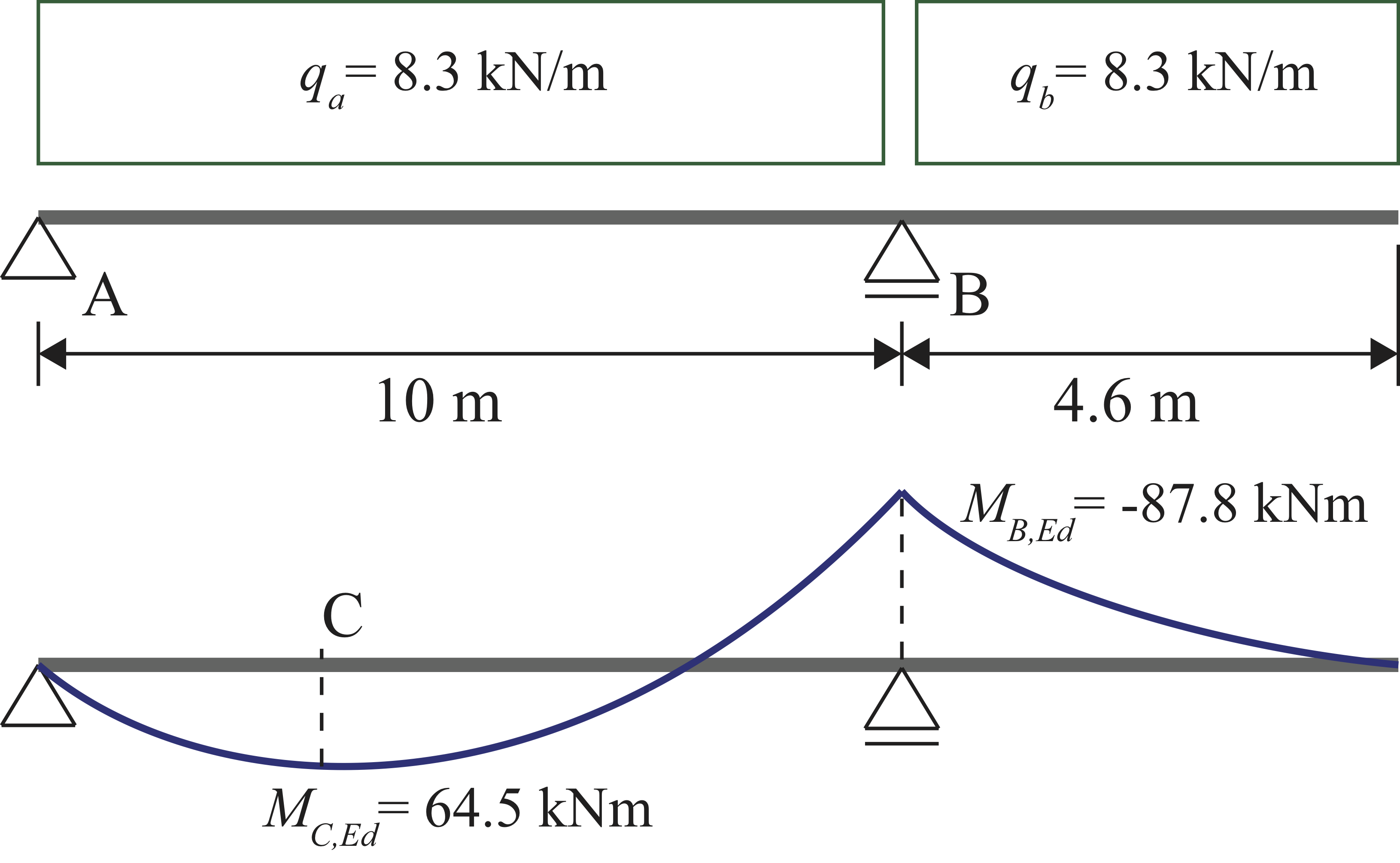
Bending moment in C: \( \gamma_{G,sup} \) is applied to the self-weight at both spans.
Eq.(6.10a) of NS EN 1990:2002 $$ \begin{array}{l} q_{a,d}=\gamma_{G,sup}g_k+\psi_{0,Q}\cdot\gamma_Q \cdot q_k=1.35\cdot 2+0.7\cdot 1.5\cdot 4=6.9 \text{kN}/\text{m}\\ q_{b,d}=\gamma_{G,sup}g_k+\psi_{0,Q}\cdot\gamma_Q \cdot q_k=1.35\cdot 2+0.7\cdot0\cdot 4=2.7 \text{kN}/\text{m} \end{array} $$ Eq.(6.10b) of NS EN 1990:2002 $$ \begin{array}{l} q_{a,d}=\xi\gamma_{G,sup}g_k+\gamma_Q q_k=0.89\cdot 1.35\cdot 2+1.5\cdot 4=8.3 \text{kN}/\text{m}\\ q_{b,d}=\xi\gamma_{G,sup}g_k+\gamma_Q q_k=0.89\cdot 1.35\cdot 2+0\cdot 4=2.3 \text{kN}/\text{m} \end{array} $$
The design bending moment at an intermediate point of the Span 1 is calculated as follows. The reaction at the support A is calculated by using Eq.\eqref{eq:eq1}. The bending moment at a distance \( x \) from the support A is given by:
$$ \begin{equation} \label{eq:eq11} M(x)=R_A x-q_a \dfrac{x^2}{2} \end{equation} $$The maximum moment is found setting the derivative of Eq.\eqref{eq:eq11} to zero:
$$ \begin{array}{l} \dfrac{\text{d}M(x)}{\text{d}x}=R_A-q_a x=0\\ \\ x=\dfrac{R_A}{q_a} \end{array} $$The highest moment is found for the load combination given by Eq.(6.10b). For this load combination, \( R_A \) results in 39.07 kN. The maximum moment \( M_{C,Ed} \) happens at a distance \( x= 4.7 \) m, and yields \( M_{C,Ed}=M(4.7 \text{m})=91.94 \) kNm. The results are sketched in Figure 132.
Figure 132: Design bending moment in C \( M_{C,Ed} \) for the STR limit state according to Eqs. 6.10a and 6.10b.
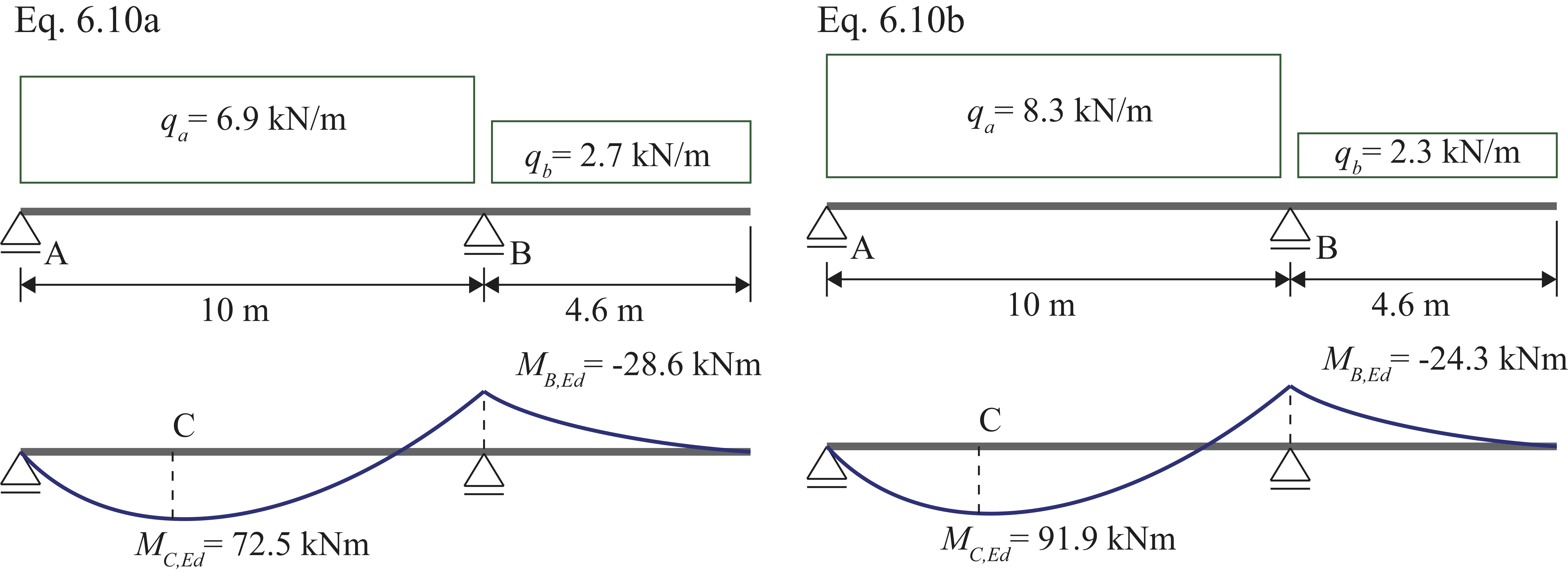
Therefore, the design bending moment of the beam is \( M_{Ed}=\max\{\vert M_{B,Ed}\vert,\vert M_{C,Ed} \vert\}=91.94 \) kNm.